
User Manual


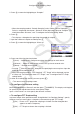


Table Of Contents
- Inhalt
- Einführung – Bitte dieses Kapitel zuerst durchlesen
- Kapitel 1 Grundlegende Operation
- Kapitel 2 Manuelle Berechnungen
- 1. Grundrechenarten
- 2. Spezielle Taschenrechnerfunktionen
- 3. Festlegung des Winkelmodus und des Anzeigeformats (SET UP)
- 4. Funktionsberechnungen
- 5. Numerische Berechnungen
- 6. Rechnen mit komplexen Zahlen
- 7. Rechnen mit (ganzen) Binär-, Oktal-, Dezimal- und Hexadezimalzahlen
- 8. Matrizenrechnung
- 9. Vektorrechnung
- 10. Umrechnen von Maßeinheiten
- Kapitel 3 Listenoperationen
- Kapitel 4 Lösung von Gleichungen
- Kapitel 5 Grafische Darstellungen
- 1. Graphenbeispiele
- 2. Voreinstellungen verschiedenster Art für eine optimale Graphenanzeige
- 3. Zeichnen eines Graphen
- 4. Speichern und Aufrufen von Inhalten des Graphenbildschirms
- 5. Zeichnen von zwei Graphen im gleichen Display
- 6. Manuelle grafische Darstellung
- 7. Verwendung von Wertetabellen
- 8. Ändern eines Graphen
- 9. Dynamischer Graph (Graphanimation einer Kurvenschar)
- 10. Grafische Darstellung von Rekursionsformeln
- 11. Grafische Darstellung eines Kegelschnitts
- 12. Zeichnen von Punkten, Linien und Text im Graphenbildschirm (Sketch)
- 13. Funktionsanalyse (Kurvendiskussion)
- Kapitel 6 Statistische Grafiken und Berechnungen
- 1. Vor dem Ausführen statistischer Berechnungen
- 2. Berechnungen und grafische Darstellungen mit einer eindimensionalen Stichprobe
- 3. Berechnungen und grafische Darstellungen mit einer zweidimensionalen Stichprobe (Ausgleichungsrechnung)
- 4. Ausführung statistischer Berechnungen und Ermittlung von Wahrscheinlichkeiten
- 5. Tests
- 6. Konfidenzintervall
- 7. Wahrscheinlichkeitsverteilungen
- 8. Ein- und Ausgabebedingungen für statistische Testverfahren, Konfidenzintervalle und Wahrscheinlichkeitsverteilungen
- 9. Statistikformeln
- Kapitel 7 Finanzmathematik
- 1. Vor dem Ausführen finanzmathematischer Berechnungen
- 2. Einfache Kapitalverzinsung
- 3. Kapitalverzinsung mit Zinseszins
- 4. Cashflow-Berechnungen (Investitionsrechnung)
- 5. Tilgungsberechnungen (Amortisation)
- 6. Zinssatz-Umrechnung
- 7. Herstellungskosten, Verkaufspreis, Gewinnspanne
- 8. Tages/Datums-Berechnungen
- 9. Abschreibung
- 10. Anleihenberechnungen
- 11. Finanzmathematik unter Verwendung von Funktionen
- Kapitel 8 Programmierung
- 1. Grundlegende Programmierschritte
- 2. Program-Menü-Funktionstasten
- 3. Editieren von Programminhalten
- 4. Programmverwaltung
- 5. Befehlsreferenz
- 6. Verwendung von Rechnerbefehlen in Programmen
- 7. Program-Menü-Befehlsliste
- 8. CASIO-Rechner für wissenschaftliche Funktionswertberechnungen Spezielle Befehle <=> Textkonvertierungstabelle
- 9. Programmbibliothek
- Kapitel 9 Tabellenkalkulation
- 1. Grundlagen der Tabellenkalkulation und das Funktionsmenü
- 2. Grundlegende Operationen in der Tabellenkalkulation
- 3. Verwenden spezieller Befehle des Spreadsheet -Menüs
- 4. Bedingte Formatierung
- 5. Zeichnen von statistischen Graphen sowie Durchführen von statistischen Berechnungen und Regressionsanalysen
- 6. Speicher des Spreadsheet -Menüs
- Kapitel 10 eActivity
- Kapitel 11 Speicherverwalter
- Kapitel 12 Systemverwalter
- Kapitel 13 Datentransfer
- Kapitel 14 Geometrie
- Kapitel 15 Picture Plot
- Kapitel 16 3D Graph-Funktion
- Kapitel 17 Python (nur fx-CG50, fx-CG50 AU)
- Anhang
- Prüfungsmodi
- E-CON4 Application (English)
- 1. E-CON4 Mode Overview
- 2. Sampling Screen
- 3. Auto Sensor Detection (CLAB Only)
- 4. Selecting a Sensor
- 5. Configuring the Sampling Setup
- 6. Performing Auto Sensor Calibration and Zero Adjustment
- 7. Using a Custom Probe
- 8. Using Setup Memory
- 9. Starting a Sampling Operation
- 10. Using Sample Data Memory
- 11. Using the Graph Analysis Tools to Graph Data
- 12. Graph Analysis Tool Graph Screen Operations
- 13. Calling E-CON4 Functions from an eActivity
ε-13
Configuring the Sampling Setup
5. Press c to move the highlighting to “Samples”.
When the sampling mode is “Periodic Sampling” and a CMA or Vernier Photogate
Pulley is assigned to the channel, “Distance” will be displayed in place of “Samples”. For
information about “Distance”, see “To configure the Distance setting” below.
6. Press e.
This displays a dialog box for specifying the number of samples.
7. Input the number of samples and then press w.
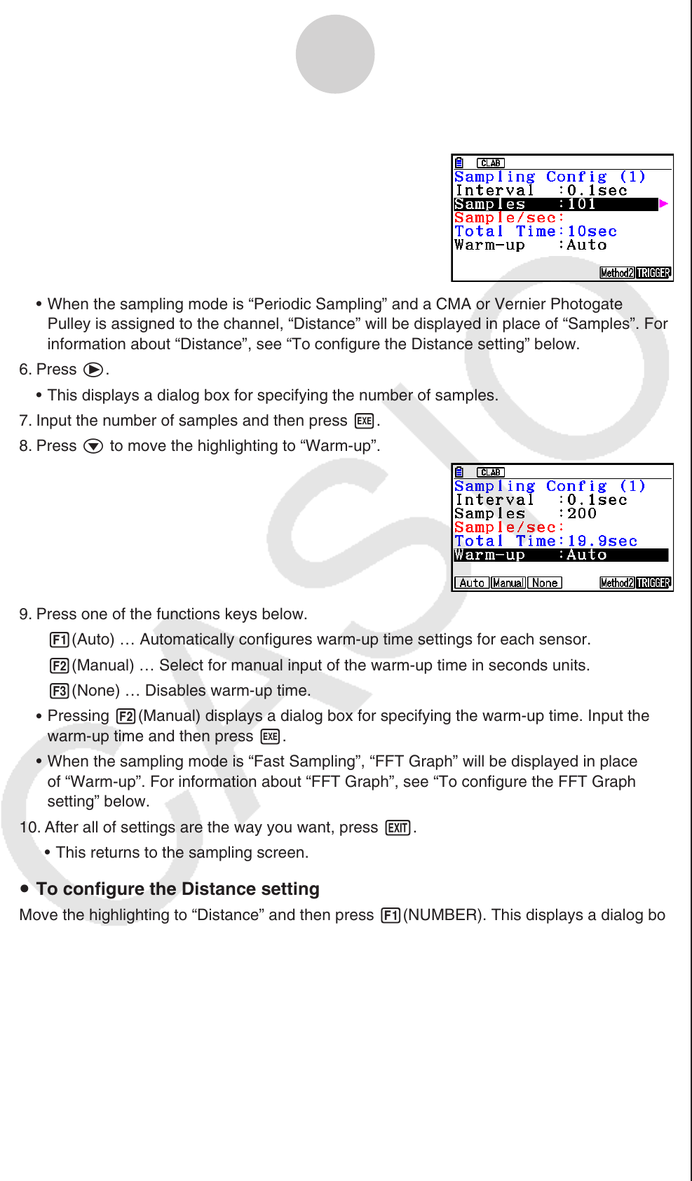
8. Press c to move the highlighting to “Warm-up”.
9. Press one of the functions keys below.
1(Auto) … Automatically configures warm-up time settings for each sensor.
2(Manual) … Select for manual input of the warm-up time in seconds units.
3(None) … Disables warm-up time.
Pressing 2(Manual) displays a dialog box for specifying the warm-up time. Input the
warm-up time and then press w.
When the sampling mode is “Fast Sampling”, “FFT Graph” will be displayed in place
of “Warm-up”. For information about “FFT Graph”, see “To configure the FFT Graph
setting” below.
10. After all of settings are the way you want, press J.
This returns to the sampling screen.
To configure the Distance setting
Move the highlighting to “Distance” and then press 1(NUMBER). This displays a dialog box
for specifying the drop distance for the smart pulley weight.
Input a value from 0.1 to 4.0 to specify the distance in meters.
To configure FFT Graph setting
In place of step 9 of the procedure under “Using Method 1 to Configure Settings”, specify
whether or not you want to draw a frequency characteristics graph (FFT Graph).
1(On) ... Draws an FFT graph after sampling is finished. Use the dialog box that
appears to select a frequency.
2(Off) ... FFT Graph no drawn after sampling is finished.
•
•
•
•
•
u
u