
User Manual
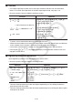
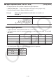
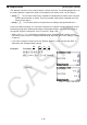


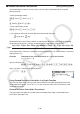
Table Of Contents
- Contents
- Getting Acquainted — Read This First!
- Chapter 1 Basic Operation
- Chapter 2 Manual Calculations
- 1. Basic Calculations
- 2. Special Functions
- 3. Specifying the Angle Unit and Display Format
- 4. Function Calculations
- 5. Numerical Calculations
- 6. Complex Number Calculations
- 7. Binary, Octal, Decimal, and Hexadecimal Calculations with Integers
- 8. Matrix Calculations
- 9. Vector Calculations
- 10. Metric Conversion Calculations
- Chapter 3 List Function
- Chapter 4 Equation Calculations
- Chapter 5 Graphing
- 1. Sample Graphs
- 2. Controlling What Appears on a Graph Screen
- 3. Drawing a Graph
- 4. Saving and Recalling Graph Screen Contents
- 5. Drawing Two Graphs on the Same Screen
- 6. Manual Graphing
- 7. Using Tables
- 8. Modifying a Graph
- 9. Dynamic Graphing
- 10. Graphing a Recursion Formula
- 11. Graphing a Conic Section
- 12. Drawing Dots, Lines, and Text on the Graph Screen (Sketch)
- 13. Function Analysis
- Chapter 6 Statistical Graphs and Calculations
- 1. Before Performing Statistical Calculations
- 2. Calculating and Graphing Single-Variable Statistical Data
- 3. Calculating and Graphing Paired-Variable Statistical Data (Curve Fitting)
- 4. Performing Statistical Calculations
- 5. Tests
- 6. Confidence Interval
- 7. Distribution
- 8. Input and Output Terms of Tests, Confidence Interval, and Distribution
- 9. Statistic Formula
- Chapter 7 Financial Calculation
- Chapter 8 Programming
- Chapter 9 Spreadsheet
- Chapter 10 eActivity
- Chapter 11 Memory Manager
- Chapter 12 System Manager
- Chapter 13 Data Communication
- Chapter 14 Geometry
- Chapter 15 Picture Plot
- Chapter 16 3D Graph Function
- Appendix
- Examination Mode
- E-CON4 Application (English)
- 1. E-CON4 Mode Overview
- 2. Sampling Screen
- 3. Auto Sensor Detection (CLAB Only)
- 4. Selecting a Sensor
- 5. Configuring the Sampling Setup
- 6. Performing Auto Sensor Calibration and Zero Adjustment
- 7. Using a Custom Probe
- 8. Using Setup Memory
- 9. Starting a Sampling Operation
- 10. Using Sample Data Memory
- 11. Using the Graph Analysis Tools to Graph Data
- 12. Graph Analysis Tool Graph Screen Operations
- 13. Calling E-CON4 Functions from an eActivity
2-31
k Integration Calculations [OPTN]-[CALC]-[∫dx]
To perform integration calculations, first display the function analysis menu and then input the
values using the syntax below.
<Math input/output mode>
K4(CALC)4(∫d
x) f(x)e a f b
or
4(MATH)6(g)1(∫d
x) f(x)e a f b
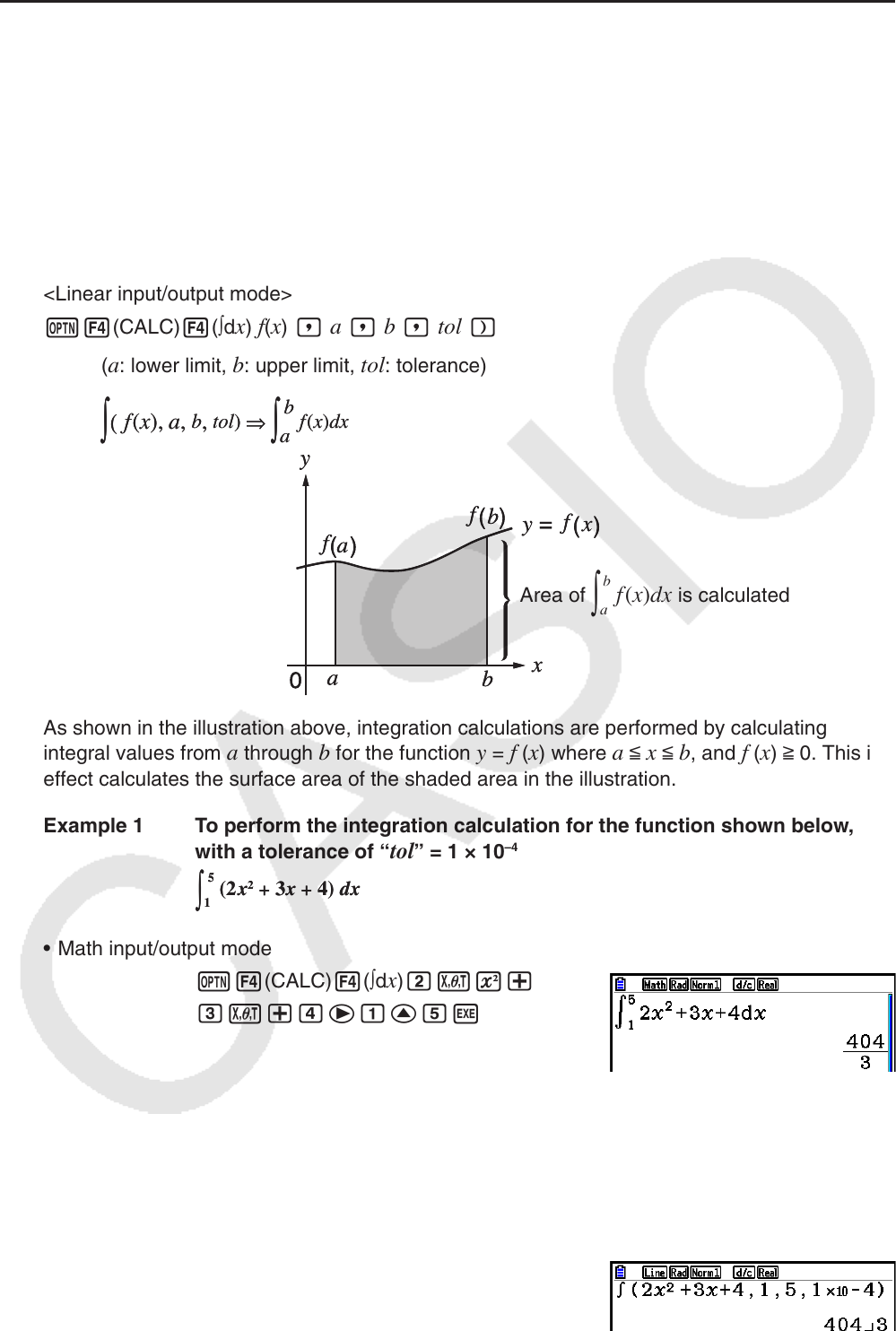
<Linear input/output mode>
K4(CALC)4(∫d
x) f(x) , a , b , tol )
(
a
: lower limit,
b
: upper limit,
tol
: tolerance)
Area of
∫
a
b
f
(
x
)
dx
is calculated
As shown in the illustration above, integration calculations are performed by calculating
integral values from
a through b for the function y = f (x) where a < x < b, and f (x) > 0. This in
effect calculates the surface area of the shaded area in the illustration.
Example 1 To perform the integration calculation for the function shown below,
with a tolerance of “
tol” = 1 × 10
–4
• Math input/output mode
K4(CALC)4(∫d
x)cvx+
dv+eebffw
• Linear input/output mode
Input the function
f
(x).
AK4(CALC)4(∫d
x)cvx+dv+e,
Input the lower limit, upper limit, and the tolerance value.
b,f,b5-e)w
∫
(
f
(
x
),
a
,
b
,
tol
)
⇒
∫
a
b
f
(
x
)
dx
∫
(
f
(
x
),
a
,
b
,
tol
)
⇒
∫
a
b
f
(
x
)
dx
∫
1
5
(2x
2
+ 3x + 4) dx
∫
1
5
(2x
2
+ 3x + 4) dx