
User Manual

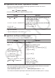
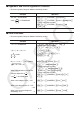

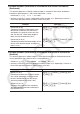

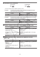
Table Of Contents
- Contents
- Getting Acquainted — Read This First!
- Chapter 1 Basic Operation
- Chapter 2 Manual Calculations
- 1. Basic Calculations
- 2. Special Functions
- 3. Specifying the Angle Unit and Display Format
- 4. Function Calculations
- 5. Numerical Calculations
- 6. Complex Number Calculations
- 7. Binary, Octal, Decimal, and Hexadecimal Calculations with Integers
- 8. Matrix Calculations
- 9. Vector Calculations
- 10. Metric Conversion Calculations
- Chapter 3 List Function
- Chapter 4 Equation Calculations
- Chapter 5 Graphing
- 1. Sample Graphs
- 2. Controlling What Appears on a Graph Screen
- 3. Drawing a Graph
- 4. Saving and Recalling Graph Screen Contents
- 5. Drawing Two Graphs on the Same Screen
- 6. Manual Graphing
- 7. Using Tables
- 8. Modifying a Graph
- 9. Dynamic Graphing
- 10. Graphing a Recursion Formula
- 11. Graphing a Conic Section
- 12. Drawing Dots, Lines, and Text on the Graph Screen (Sketch)
- 13. Function Analysis
- Chapter 6 Statistical Graphs and Calculations
- 1. Before Performing Statistical Calculations
- 2. Calculating and Graphing Single-Variable Statistical Data
- 3. Calculating and Graphing Paired-Variable Statistical Data (Curve Fitting)
- 4. Performing Statistical Calculations
- 5. Tests
- 6. Confidence Interval
- 7. Distribution
- 8. Input and Output Terms of Tests, Confidence Interval, and Distribution
- 9. Statistic Formula
- Chapter 7 Financial Calculation
- Chapter 8 Programming
- Chapter 9 Spreadsheet
- Chapter 10 eActivity
- Chapter 11 Memory Manager
- Chapter 12 System Manager
- Chapter 13 Data Communication
- Chapter 14 Geometry
- Chapter 15 Picture Plot
- Chapter 16 3D Graph Function
- Appendix
- Examination Mode
- E-CON4 Application (English)
- 1. E-CON4 Mode Overview
- 2. Sampling Screen
- 3. Auto Sensor Detection (CLAB Only)
- 4. Selecting a Sensor
- 5. Configuring the Sampling Setup
- 6. Performing Auto Sensor Calibration and Zero Adjustment
- 7. Using a Custom Probe
- 8. Using Setup Memory
- 9. Starting a Sampling Operation
- 10. Using Sample Data Memory
- 11. Using the Graph Analysis Tools to Graph Data
- 12. Graph Analysis Tool Graph Screen Operations
- 13. Calling E-CON4 Functions from an eActivity
2-16
k Trigonometric and Inverse Trigonometric Functions
• Be sure to set the angle unit before performing trigonometric function and inverse
trigonometric function calculations.
• Be sure to specify Comp for Mode in the Setup screen.
Example Operation
cos (
π
3
rad) =
2
1
(0.5)
!m(SET UP)cccccc2(Rad)J
c'!5(π)c3w
<Linear input/output mode>
c(!5(π)/3)w
2
•
sin 45° × cos 65° = 0.5976724775
!m(SET UP)cccccc1(Deg)J
2*s45*c65w*
1
sin
–1
0.5 = 30°
(x when sinx = 0.5)
!s(sin
–1
) 0.5*
2
w
*
1
* can be omitted.
*
2
Input of leading zero is not necessary.
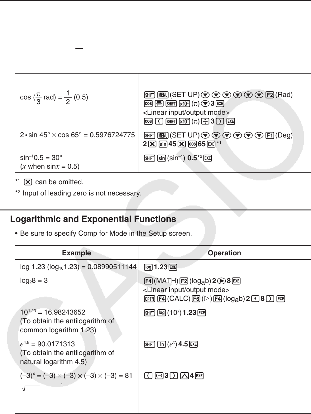
k Logarithmic and Exponential Functions
• Be sure to specify Comp for Mode in the Setup screen.
Example Operation
log 1.23 (log
10
1.23) = 0.08990511144
l1.23w
log
2
8 = 3
4(MATH)2(log
a
b) 2e8w
<Linear input/output mode>
K4(CALC)6(g)4(log
a
b) 2,8)w
10
1.23
= 16.98243652
(To obtain the antilogarithm of
common logarithm 1.23)
!l(10
x
) 1.23w
e
4.5
= 90.0171313
(To obtain the antilogarithm of
natural logarithm 4.5)
!I(e
x
) 4.5w
(–3)
4
= (–3) × (–3) × (–3) × (–3) = 81
(-3)M4w
7
123 (= 123
1
7
) = 1.988647795
!M(
x
') 7e123w
<Linear input/output mode>
7!M(
x
')123w
• The Linear input/output mode and Math input/output mode produce different results when
two or more powers are input in series, like: 2 M 3 M 2.
Linear input/output mode: 2^3^2 = 64 Math input/output mode:
2
3
2
= 512
This is because the Math input/output mode internally treats the above input as: 2^(3^(2)).
(90° = radians = 100 grads)
π
2
(90° = radians = 100 grads)
π
2