
User Manual
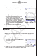
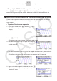
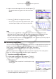
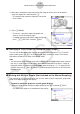
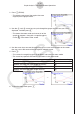
Table Of Contents
- Contents
- Getting Acquainted — Read This First!
- Chapter 1 Basic Operation
- Chapter 2 Manual Calculations
- 1. Basic Calculations
- 2. Special Functions
- 3. Specifying the Angle Unit and Display Format
- 4. Function Calculations
- 5. Numerical Calculations
- 6. Complex Number Calculations
- 7. Binary, Octal, Decimal, and Hexadecimal Calculations with Integers
- 8. Matrix Calculations
- 9. Vector Calculations
- 10. Metric Conversion Calculations
- Chapter 3 List Function
- Chapter 4 Equation Calculations
- Chapter 5 Graphing
- 1. Sample Graphs
- 2. Controlling What Appears on a Graph Screen
- 3. Drawing a Graph
- 4. Saving and Recalling Graph Screen Contents
- 5. Drawing Two Graphs on the Same Screen
- 6. Manual Graphing
- 7. Using Tables
- 8. Modifying a Graph
- 9. Dynamic Graphing
- 10. Graphing a Recursion Formula
- 11. Graphing a Conic Section
- 12. Drawing Dots, Lines, and Text on the Graph Screen (Sketch)
- 13. Function Analysis
- Chapter 6 Statistical Graphs and Calculations
- 1. Before Performing Statistical Calculations
- 2. Calculating and Graphing Single-Variable Statistical Data
- 3. Calculating and Graphing Paired-Variable Statistical Data (Curve Fitting)
- 4. Performing Statistical Calculations
- 5. Tests
- 6. Confidence Interval
- 7. Distribution
- 8. Input and Output Terms of Tests, Confidence Interval, and Distribution
- 9. Statistic Formula
- Chapter 7 Financial Calculation
- Chapter 8 Programming
- Chapter 9 Spreadsheet
- Chapter 10 eActivity
- Chapter 11 Memory Manager
- Chapter 12 System Manager
- Chapter 13 Data Communication
- Chapter 14 Geometry
- Chapter 15 Picture Plot
- Chapter 16 3D Graph Function
- Appendix
- Examination Mode
- E-CON4 Application (English)
- 1. E-CON4 Mode Overview
- 2. Sampling Screen
- 3. Auto Sensor Detection (CLAB Only)
- 4. Selecting a Sensor
- 5. Configuring the Sampling Setup
- 6. Performing Auto Sensor Calibration and Zero Adjustment
- 7. Using a Custom Probe
- 8. Using Setup Memory
- 9. Starting a Sampling Operation
- 10. Using Sample Data Memory
- 11. Using the Graph Analysis Tools to Graph Data
- 12. Graph Analysis Tool Graph Screen Operations
- 13. Calling E-CON4 Functions from an eActivity
ε-45
Graph Analysis Tool Graph Screen Operations
6. Input a value in the range of 1 to 10, and then press w.
• The graph relation list appears with the calculation
result.
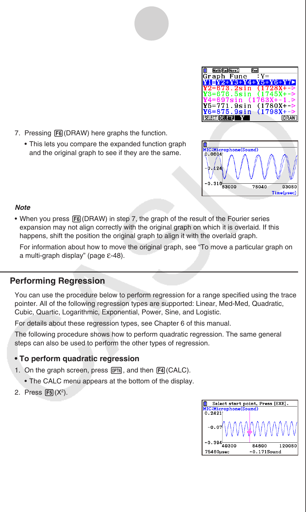
7. Pressing 6(DRAW) here graphs the function.
• This lets you compare the expanded function graph
and the original graph to see if they are the same.
Note
• When you press 6(DRAW) in step 7, the graph of the result of the Fourier series
expansion may not align correctly with the original graph on which it is overlaid. If this
happens, shift the position the original graph to align it with the overlaid graph.
For information about how to move the original graph, see “To move a particular graph on
a multi-graph display” (page
ε-48).
k Performing Regression
You can use the procedure below to perform regression for a range specified using the trace
pointer. All of the following regression types are supported: Linear, Med-Med, Quadratic,
Cubic, Quartic, Logarithmic, Exponential, Power, Sine, and Logistic.
For details about these regression types, see Chapter 6 of this manual.
The following procedure shows how to perform quadratic regression. The same general
steps can also be used to perform the other types of regression.
• To perform quadratic regression
1. On the graph screen, press K, and then 4(CALC).
• The CALC menu appears at the bottom of the display.
2. Press 5(X
2
).
• This displays the trace pointer for selecting the range
on the graph.
3. Move the trace pointer to the start point of the range for which you want to perform
quadratic regression, and then press w.