
User Manual
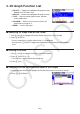
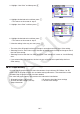
Table Of Contents
- Contents
- Getting Acquainted — Read This First!
- Chapter 1 Basic Operation
- Chapter 2 Manual Calculations
- 1. Basic Calculations
- 2. Special Functions
- 3. Specifying the Angle Unit and Display Format
- 4. Function Calculations
- 5. Numerical Calculations
- 6. Complex Number Calculations
- 7. Binary, Octal, Decimal, and Hexadecimal Calculations with Integers
- 8. Matrix Calculations
- 9. Vector Calculations
- 10. Metric Conversion Calculations
- Chapter 3 List Function
- Chapter 4 Equation Calculations
- Chapter 5 Graphing
- 1. Sample Graphs
- 2. Controlling What Appears on a Graph Screen
- 3. Drawing a Graph
- 4. Saving and Recalling Graph Screen Contents
- 5. Drawing Two Graphs on the Same Screen
- 6. Manual Graphing
- 7. Using Tables
- 8. Modifying a Graph
- 9. Dynamic Graphing
- 10. Graphing a Recursion Formula
- 11. Graphing a Conic Section
- 12. Drawing Dots, Lines, and Text on the Graph Screen (Sketch)
- 13. Function Analysis
- Chapter 6 Statistical Graphs and Calculations
- 1. Before Performing Statistical Calculations
- 2. Calculating and Graphing Single-Variable Statistical Data
- 3. Calculating and Graphing Paired-Variable Statistical Data (Curve Fitting)
- 4. Performing Statistical Calculations
- 5. Tests
- 6. Confidence Interval
- 7. Distribution
- 8. Input and Output Terms of Tests, Confidence Interval, and Distribution
- 9. Statistic Formula
- Chapter 7 Financial Calculation
- Chapter 8 Programming
- Chapter 9 Spreadsheet
- Chapter 10 eActivity
- Chapter 11 Memory Manager
- Chapter 12 System Manager
- Chapter 13 Data Communication
- Chapter 14 Geometry
- Chapter 15 Picture Plot
- Chapter 16 3D Graph Function
- Appendix
- Examination Mode
- E-CON4 Application (English)
- 1. E-CON4 Mode Overview
- 2. Sampling Screen
- 3. Auto Sensor Detection (CLAB Only)
- 4. Selecting a Sensor
- 5. Configuring the Sampling Setup
- 6. Performing Auto Sensor Calibration and Zero Adjustment
- 7. Using a Custom Probe
- 8. Using Setup Memory
- 9. Starting a Sampling Operation
- 10. Using Sample Data Memory
- 11. Using the Graph Analysis Tools to Graph Data
- 12. Graph Analysis Tool Graph Screen Operations
- 13. Calling E-CON4 Functions from an eActivity
15-18
5. Common Functions with the Graph Mode
On the Picture Plot screen, !1 to 5 function menu items are the same as those in the
Graph mode. See the pages below for more information.
• !1(TRACE) ... “Reading Coordinates on a Graph Line” (page 5-54)
• !2(ZOOM) ... “Zoom” (page 5-8)
• !3(V-WIN) ... “V-Window (View Window) Settings” (page 5-5)
• !4(SKETCH) ... “Drawing Dots, Lines, and Text on the Graph Screen (Sketch)” (page
5-52)
• !5(G-SOLVE) ... “Analyzing Graphs (G-SOLVE Menu)” (page 5-56)
Note
After you start a trace operation by pressing !1(TRACE), you can change the color of the
plot where the trace pointer is currently located. Perform the following steps to change the plot
color.
1. While the Picture Plot screen contains plotted points, press !1(TRACE).
• This causes a trace pointer to appear at the first point that was plotted on the image.
• If there are both plots and a graph on the Picture Plot screen, pressing !1(TRACE)
will cause the trace pointer to appear on the graph first. In this case, use f and c to
move the trace pointer between the graph and the plots.
2. Use e and d to move the trace pointer to the plot whose color you want to change.
3. Press !f(FORMAT) to display the FORMAT dialog box.
4. Use the cursor keys to move the highlighting to the desired color and then press w.
• The color you change to is also reflected in the text color of the corresponding plot data.