
User Manual
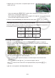
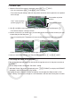
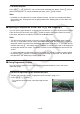

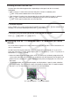
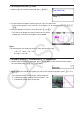
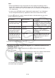
Table Of Contents
- Contents
- Getting Acquainted — Read This First!
- Chapter 1 Basic Operation
- Chapter 2 Manual Calculations
- 1. Basic Calculations
- 2. Special Functions
- 3. Specifying the Angle Unit and Display Format
- 4. Function Calculations
- 5. Numerical Calculations
- 6. Complex Number Calculations
- 7. Binary, Octal, Decimal, and Hexadecimal Calculations with Integers
- 8. Matrix Calculations
- 9. Vector Calculations
- 10. Metric Conversion Calculations
- Chapter 3 List Function
- Chapter 4 Equation Calculations
- Chapter 5 Graphing
- 1. Sample Graphs
- 2. Controlling What Appears on a Graph Screen
- 3. Drawing a Graph
- 4. Saving and Recalling Graph Screen Contents
- 5. Drawing Two Graphs on the Same Screen
- 6. Manual Graphing
- 7. Using Tables
- 8. Modifying a Graph
- 9. Dynamic Graphing
- 10. Graphing a Recursion Formula
- 11. Graphing a Conic Section
- 12. Drawing Dots, Lines, and Text on the Graph Screen (Sketch)
- 13. Function Analysis
- Chapter 6 Statistical Graphs and Calculations
- 1. Before Performing Statistical Calculations
- 2. Calculating and Graphing Single-Variable Statistical Data
- 3. Calculating and Graphing Paired-Variable Statistical Data (Curve Fitting)
- 4. Performing Statistical Calculations
- 5. Tests
- 6. Confidence Interval
- 7. Distribution
- 8. Input and Output Terms of Tests, Confidence Interval, and Distribution
- 9. Statistic Formula
- Chapter 7 Financial Calculation
- Chapter 8 Programming
- Chapter 9 Spreadsheet
- Chapter 10 eActivity
- Chapter 11 Memory Manager
- Chapter 12 System Manager
- Chapter 13 Data Communication
- Chapter 14 Geometry
- Chapter 15 Picture Plot
- Chapter 16 3D Graph Function
- Appendix
- Examination Mode
- E-CON4 Application (English)
- 1. E-CON4 Mode Overview
- 2. Sampling Screen
- 3. Auto Sensor Detection (CLAB Only)
- 4. Selecting a Sensor
- 5. Configuring the Sampling Setup
- 6. Performing Auto Sensor Calibration and Zero Adjustment
- 7. Using a Custom Probe
- 8. Using Setup Memory
- 9. Starting a Sampling Operation
- 10. Using Sample Data Memory
- 11. Using the Graph Analysis Tools to Graph Data
- 12. Graph Analysis Tool Graph Screen Operations
- 13. Calling E-CON4 Functions from an eActivity
15-10
u To delete all plots
Press K6(g)4(DELETE), and a confirmation dialog box will appear. Press 1(Yes) to
delete all of the plots. To cancel the delete operation, press 6(No) instead.
Note
• In addition to using the plot list screen to delete all plots, you also can sequentially delete
plots one-by-one, starting from the last point plotted. See “Deleting the Last Plot Data Line”
(page 15-14).
k Inputting an Expression of the Form Y=f(x) and Graphing It
You can draw a graph based on an expression with the form Y=f(x) on the Picture Plot screen.
From the Picture Plot screen, press K4(DefG) to display the graph relation list screen.
From there, operations are identical to those in the Graph mode.
Note
• The data on the graph relation list screen is shared with the Graph mode. Note, however,
that only Y= type graphs can be used in the Picture Plot mode. Because of this, calling up
the graph relation list screen from the Picture Plot mode will display a “Y” (Y= type) item for
function menu key 3. Also note that the 5(MODIFY) function menu item is not displayed
on the graph relation list screen. The Modify function can be executed from the Picture Plot
screen.
• Y= type expressions on the graph relation list screen that include variables can be modified
by pressing K5(MODIFY) while the Picture Plot screen is displayed. For details about
this operation, see “Modifying a Graph” (page 5-38).
k Using Regression Graphs
You can perform regression calculation based on plotted coordinate values and draw a
regression graph.
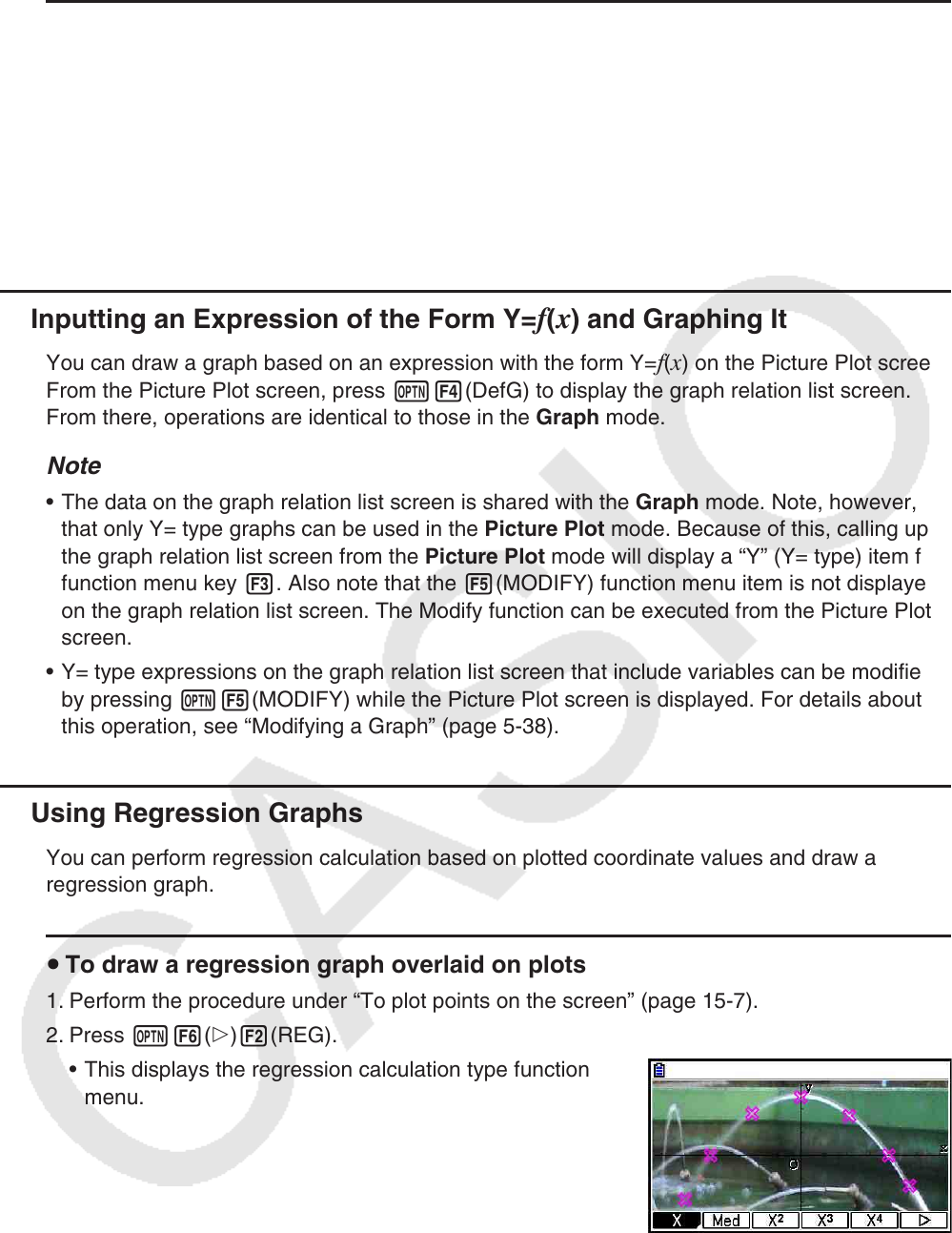
u To draw a regression graph overlaid on plots
1. Perform the procedure under “To plot points on the screen” (page 15-7).
2. Press K6(g)2(REG).
• This displays the regression calculation type function
menu.