User Manual

15-7
u To save a file under a different name
1. While the Picture Plot screen is displayed, press K1(FILE)3(SAVE
•
AS).
• This displays a folder selection screen.
2. Specify the folder you want.
• Highlight ROOT to save the file to the root directory.
• To save the file in a specific folder, use f and c to move the highlighting to the desired
folder and then press 1(OPEN).
3. Press 1(SAVE
•
AS).
4. On the File Name dialog box that appears, enter a name up to eight characters long and
then press w.
3. Using the Plot Function
You can plot points on the screen, overlay them with a graph of an expression in the form
Y=
f(x), and draw a regression graph that approximates the plots.
k Plotting Points
u To plot points on the screen
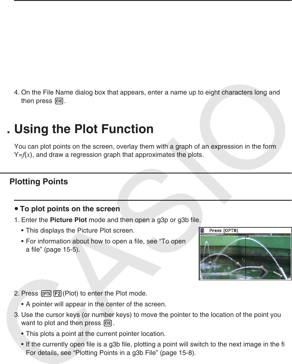
1. Enter the Picture Plot mode and then open a g3p or g3b file.
• This displays the Picture Plot screen.
• For information about how to open a file, see “To open
a file” (page 15-5).
2. Press K2(Plot) to enter the Plot mode.
• A pointer will appear in the center of the screen.
3. Use the cursor keys (or number keys) to move the pointer to the location of the point you
want to plot and then press w.
• This plots a point at the current pointer location.
• If the currently open file is a g3b file, plotting a point will switch to the next image in the file.
For details, see “Plotting Points in a g3b File” (page 15-8).
• To delete the last point you plotted, press K2(UNDO).
• For information about using the number keys to move the pointer to a particular location,
see “To make the pointer jump to a particular location” (page 15-8).