
User Manual
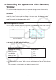
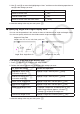
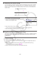
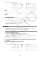
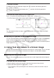
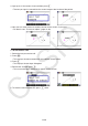
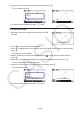

Table Of Contents
- Contents
- Getting Acquainted — Read This First!
- Chapter 1 Basic Operation
- Chapter 2 Manual Calculations
- 1. Basic Calculations
- 2. Special Functions
- 3. Specifying the Angle Unit and Display Format
- 4. Function Calculations
- 5. Numerical Calculations
- 6. Complex Number Calculations
- 7. Binary, Octal, Decimal, and Hexadecimal Calculations with Integers
- 8. Matrix Calculations
- 9. Vector Calculations
- 10. Metric Conversion Calculations
- Chapter 3 List Function
- Chapter 4 Equation Calculations
- Chapter 5 Graphing
- 1. Sample Graphs
- 2. Controlling What Appears on a Graph Screen
- 3. Drawing a Graph
- 4. Saving and Recalling Graph Screen Contents
- 5. Drawing Two Graphs on the Same Screen
- 6. Manual Graphing
- 7. Using Tables
- 8. Modifying a Graph
- 9. Dynamic Graphing
- 10. Graphing a Recursion Formula
- 11. Graphing a Conic Section
- 12. Drawing Dots, Lines, and Text on the Graph Screen (Sketch)
- 13. Function Analysis
- Chapter 6 Statistical Graphs and Calculations
- 1. Before Performing Statistical Calculations
- 2. Calculating and Graphing Single-Variable Statistical Data
- 3. Calculating and Graphing Paired-Variable Statistical Data (Curve Fitting)
- 4. Performing Statistical Calculations
- 5. Tests
- 6. Confidence Interval
- 7. Distribution
- 8. Input and Output Terms of Tests, Confidence Interval, and Distribution
- 9. Statistic Formula
- Chapter 7 Financial Calculation
- Chapter 8 Programming
- Chapter 9 Spreadsheet
- Chapter 10 eActivity
- Chapter 11 Memory Manager
- Chapter 12 System Manager
- Chapter 13 Data Communication
- Chapter 14 Geometry
- Chapter 15 Picture Plot
- Chapter 16 3D Graph Function
- Appendix
- Examination Mode
- E-CON4 Application (English)
- 1. E-CON4 Mode Overview
- 2. Sampling Screen
- 3. Auto Sensor Detection (CLAB Only)
- 4. Selecting a Sensor
- 5. Configuring the Sampling Setup
- 6. Performing Auto Sensor Calibration and Zero Adjustment
- 7. Using a Custom Probe
- 8. Using Setup Memory
- 9. Starting a Sampling Operation
- 10. Using Sample Data Memory
- 11. Using the Graph Analysis Tools to Graph Data
- 12. Graph Analysis Tool Graph Screen Operations
- 13. Calling E-CON4 Functions from an eActivity
14-33
3. Controlling the Appearance of the Geometry
Window
This section provides information about how to control the appearance of the screen by
scrolling or zooming, and by showing or hiding axes and the grid.
Important!
Settings you configure on the Geometry mode Setup screen are applied in the Geometry
mode only. Even if another mode has settings of the same name, the Geometry mode
settings will not affect them. Conversely, changing setting with the same name in another
mode will not affect the Geometry mode settings.
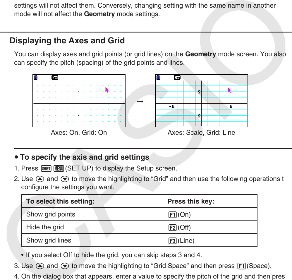
k Displaying the Axes and Grid
You can display axes and grid points (or grid lines) on the Geometry mode screen. You also
can specify the pitch (spacing) of the grid points and lines.
→
Axes: On, Grid: On Axes: Scale, Grid: Line
u To specify the axis and grid settings
1. Press !m(SET UP) to display the Setup screen.
2. Use f and c to move the highlighting to “Grid” and then use the following operations to
configure the settings you want.
To select this setting: Press this key:
Show grid points
1(On)
Hide the grid
2(Off)
Show grid lines
3(Line)
• If you select Off to hide the grid, you can skip steps 3 and 4.
3. Use f and c to move the highlighting to “Grid Space” and then press 1(Space).
4. On the dialog box that appears, enter a value to specify the pitch of the grid and then press
w.
• You can specify a value from 0.01 to 1000, in increments of 0.01.