
User Manual
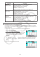
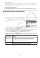
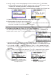
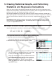
Table Of Contents
- Contents
- Getting Acquainted — Read This First!
- Chapter 1 Basic Operation
- Chapter 2 Manual Calculations
- 1. Basic Calculations
- 2. Special Functions
- 3. Specifying the Angle Unit and Display Format
- 4. Function Calculations
- 5. Numerical Calculations
- 6. Complex Number Calculations
- 7. Binary, Octal, Decimal, and Hexadecimal Calculations with Integers
- 8. Matrix Calculations
- 9. Vector Calculations
- 10. Metric Conversion Calculations
- Chapter 3 List Function
- Chapter 4 Equation Calculations
- Chapter 5 Graphing
- 1. Sample Graphs
- 2. Controlling What Appears on a Graph Screen
- 3. Drawing a Graph
- 4. Saving and Recalling Graph Screen Contents
- 5. Drawing Two Graphs on the Same Screen
- 6. Manual Graphing
- 7. Using Tables
- 8. Modifying a Graph
- 9. Dynamic Graphing
- 10. Graphing a Recursion Formula
- 11. Graphing a Conic Section
- 12. Drawing Dots, Lines, and Text on the Graph Screen (Sketch)
- 13. Function Analysis
- Chapter 6 Statistical Graphs and Calculations
- 1. Before Performing Statistical Calculations
- 2. Calculating and Graphing Single-Variable Statistical Data
- 3. Calculating and Graphing Paired-Variable Statistical Data (Curve Fitting)
- 4. Performing Statistical Calculations
- 5. Tests
- 6. Confidence Interval
- 7. Distribution
- 8. Input and Output Terms of Tests, Confidence Interval, and Distribution
- 9. Statistic Formula
- Chapter 7 Financial Calculation
- Chapter 8 Programming
- Chapter 9 Spreadsheet
- Chapter 10 eActivity
- Chapter 11 Memory Manager
- Chapter 12 System Manager
- Chapter 13 Data Communication
- Chapter 14 Geometry
- Chapter 15 Picture Plot
- Chapter 16 3D Graph Function
- Appendix
- Examination Mode
- E-CON4 Application (English)
- 1. E-CON4 Mode Overview
- 2. Sampling Screen
- 3. Auto Sensor Detection (CLAB Only)
- 4. Selecting a Sensor
- 5. Configuring the Sampling Setup
- 6. Performing Auto Sensor Calibration and Zero Adjustment
- 7. Using a Custom Probe
- 8. Using Setup Memory
- 9. Starting a Sampling Operation
- 10. Using Sample Data Memory
- 11. Using the Graph Analysis Tools to Graph Data
- 12. Graph Analysis Tool Graph Screen Operations
- 13. Calling E-CON4 Functions from an eActivity
9-27
5. Drawing Statistical Graphs, and Performing
Statistical and Regression Calculations
When you want to check the correlation between two sets of data (such as temperature and
the price of some product), trends become easier to spot if you draw a graph that uses one set
of data as the
x -axis and the other set of data as the y -axis.
With the spreadsheet you can input the values for each set of data and draw a scatter plot or
other types of graphs. Performing regression calculations on the data will produce a regression
formula and correlation coefficient, and you can overlay a regression graph over the scatter
plot.
Spreadsheet
mode graphing, statistical calculations, and regression calculations use the
same functions as the Statistics mode. The following shows an operation example that is
unique to the Spreadsheet
mode.
k Example of Statistical Graph Operations (GRAPH Menu)
Input the following data and draw a statistical graph (scatter plot in this example).
0.5, 1.2, 2.4, 4.0, 5.2 (
x -axis data)
–2.1, 0.3, 1.5, 2.0, 2.4 (
y -axis data)
u To input data and draw a statistical graph (scatter plot)
1. Input the statistical calculation data into the spreadsheet.
• Here we will input the
x -axis data into column A, and the y -axis data into column B.
2. Select the range of cells you want to graph (A1:B5).
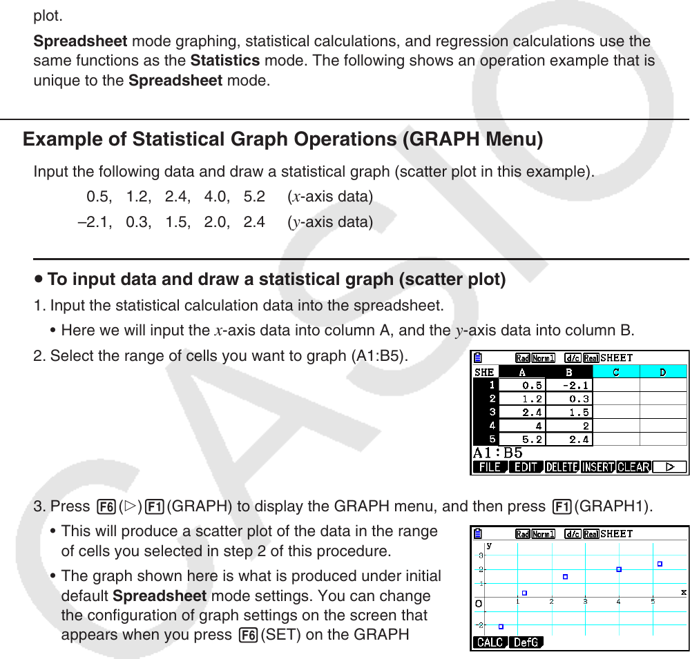
3. Press 6( g) 1(GRAPH) to display the GRAPH menu, and then press 1(GRAPH1).
• This will produce a scatter plot of the data in the range
of cells you selected in step 2 of this procedure.
• The graph shown here is what is produced under initial
default Spreadsheet
mode settings. You can change
the configuration of graph settings on the screen that
appears when you press 6(SET) on the GRAPH
menu. For details see “General Graph Settings Screen
Operations” below.