
User Manual
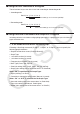
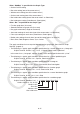
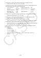
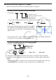
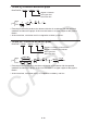
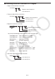
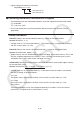
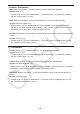
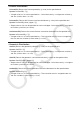
Table Of Contents
- Contents
- Getting Acquainted — Read This First!
- Chapter 1 Basic Operation
- Chapter 2 Manual Calculations
- 1. Basic Calculations
- 2. Special Functions
- 3. Specifying the Angle Unit and Display Format
- 4. Function Calculations
- 5. Numerical Calculations
- 6. Complex Number Calculations
- 7. Binary, Octal, Decimal, and Hexadecimal Calculations with Integers
- 8. Matrix Calculations
- 9. Vector Calculations
- 10. Metric Conversion Calculations
- Chapter 3 List Function
- Chapter 4 Equation Calculations
- Chapter 5 Graphing
- 1. Sample Graphs
- 2. Controlling What Appears on a Graph Screen
- 3. Drawing a Graph
- 4. Saving and Recalling Graph Screen Contents
- 5. Drawing Two Graphs on the Same Screen
- 6. Manual Graphing
- 7. Using Tables
- 8. Modifying a Graph
- 9. Dynamic Graphing
- 10. Graphing a Recursion Formula
- 11. Graphing a Conic Section
- 12. Drawing Dots, Lines, and Text on the Graph Screen (Sketch)
- 13. Function Analysis
- Chapter 6 Statistical Graphs and Calculations
- 1. Before Performing Statistical Calculations
- 2. Calculating and Graphing Single-Variable Statistical Data
- 3. Calculating and Graphing Paired-Variable Statistical Data (Curve Fitting)
- 4. Performing Statistical Calculations
- 5. Tests
- 6. Confidence Interval
- 7. Distribution
- 8. Input and Output Terms of Tests, Confidence Interval, and Distribution
- 9. Statistic Formula
- Chapter 7 Financial Calculation
- Chapter 8 Programming
- Chapter 9 Spreadsheet
- Chapter 10 eActivity
- Chapter 11 Memory Manager
- Chapter 12 System Manager
- Chapter 13 Data Communication
- Chapter 14 Geometry
- Chapter 15 Picture Plot
- Chapter 16 3D Graph Function
- Appendix
- Examination Mode
- E-CON4 Application (English)
- 1. E-CON4 Mode Overview
- 2. Sampling Screen
- 3. Auto Sensor Detection (CLAB Only)
- 4. Selecting a Sensor
- 5. Configuring the Sampling Setup
- 6. Performing Auto Sensor Calibration and Zero Adjustment
- 7. Using a Custom Probe
- 8. Using Setup Memory
- 9. Starting a Sampling Operation
- 10. Using Sample Data Memory
- 11. Using the Graph Analysis Tools to Graph Data
- 12. Graph Analysis Tool Graph Screen Operations
- 13. Calling E-CON4 Functions from an eActivity
8-39
k Using Distribution Graphs in a Program
Special commands are used to draw distribution graphs in a program.
• To draw a normal cumulative distribution graph
DrawDistNorm <Lower>, <Upper> [,
σ
, ]
Population mean *
1
Population standard deviation *
1
Data upper limit
Data lower limit
*
1
This can be omitted. Omitting these items performs the calculation using = 1 and = 0.
• Executing DrawDistNorm performs the above calculation
in accordance with the specified conditions and draws
the graph. At this time the ZLow <
x < ZUp region on the
graph is filled in.
• At the same time, the
p, ZLow, and ZUp calculation result values are assigned respectively
to variables p, ZLow, and ZUp, and p is assigned to Ans.
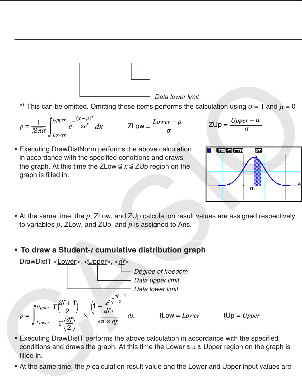
• To draw a Student- t cumulative distribution graph
DrawDistT <Lower>, <Upper>, <df>
Degree of freedom
Data upper limit
Data lower limit
• Executing DrawDistT performs the above calculation in accordance with the specified
conditions and draws the graph. At this time the Lower <
x < Upper region on the graph is
filled in.
• At the same time, the
p calculation result value and the Lower and Upper input values are
assigned respectively to variables
p , tLow, and tUp, and p is assigned to Ans.
πσ
2
p =
dx
1
e
–
2
2
σ
(x – μ)
2
μ
Upper
Lower
∫
ZUp =
σ
Upper –
μ
ZLow =
σ
Lower –
μ
πσ
2
p =
dx
1
e
–
2
2
σ
(x – μ)
2
μ
Upper
Lower
∫
ZUp =
σ
Upper –
μ
ZLow =
σ
Lower –
μ
tLow = Lower tUp = Upper
Γ
2
df + 1
df
x
2
1 +
df + 1
2
p = ×
–
Γ
2
df
dx
df
×
π
Upper
Lower
∫
tLow = Lower tUp = Upper
Γ
2
df + 1
df
x
2
1 +
df + 1
2
p = ×
–
Γ
2
df
dx
df
×
π
Upper
Lower
∫