
User Manual
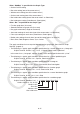
Table Of Contents
- Contents
- Getting Acquainted — Read This First!
- Chapter 1 Basic Operation
- Chapter 2 Manual Calculations
- 1. Basic Calculations
- 2. Special Functions
- 3. Specifying the Angle Unit and Display Format
- 4. Function Calculations
- 5. Numerical Calculations
- 6. Complex Number Calculations
- 7. Binary, Octal, Decimal, and Hexadecimal Calculations with Integers
- 8. Matrix Calculations
- 9. Vector Calculations
- 10. Metric Conversion Calculations
- Chapter 3 List Function
- Chapter 4 Equation Calculations
- Chapter 5 Graphing
- 1. Sample Graphs
- 2. Controlling What Appears on a Graph Screen
- 3. Drawing a Graph
- 4. Saving and Recalling Graph Screen Contents
- 5. Drawing Two Graphs on the Same Screen
- 6. Manual Graphing
- 7. Using Tables
- 8. Modifying a Graph
- 9. Dynamic Graphing
- 10. Graphing a Recursion Formula
- 11. Graphing a Conic Section
- 12. Drawing Dots, Lines, and Text on the Graph Screen (Sketch)
- 13. Function Analysis
- Chapter 6 Statistical Graphs and Calculations
- 1. Before Performing Statistical Calculations
- 2. Calculating and Graphing Single-Variable Statistical Data
- 3. Calculating and Graphing Paired-Variable Statistical Data (Curve Fitting)
- 4. Performing Statistical Calculations
- 5. Tests
- 6. Confidence Interval
- 7. Distribution
- 8. Input and Output Terms of Tests, Confidence Interval, and Distribution
- 9. Statistic Formula
- Chapter 7 Financial Calculation
- Chapter 8 Programming
- Chapter 9 Spreadsheet
- Chapter 10 eActivity
- Chapter 11 Memory Manager
- Chapter 12 System Manager
- Chapter 13 Data Communication
- Chapter 14 Geometry
- Chapter 15 Picture Plot
- Chapter 16 3D Graph Function
- Appendix
- Examination Mode
- E-CON4 Application (English)
- 1. E-CON4 Mode Overview
- 2. Sampling Screen
- 3. Auto Sensor Detection (CLAB Only)
- 4. Selecting a Sensor
- 5. Configuring the Sampling Setup
- 6. Performing Auto Sensor Calibration and Zero Adjustment
- 7. Using a Custom Probe
- 8. Using Setup Memory
- 9. Starting a Sampling Operation
- 10. Using Sample Data Memory
- 11. Using the Graph Analysis Tools to Graph Data
- 12. Graph Analysis Tool Graph Screen Operations
- 13. Calling E-CON4 Functions from an eActivity
8-38
• The following is a typical graph condition specification for a regression graph.
S-Gph1 DrawOn, Linear, List 1, List 2, List 3, Blue
The same format can be used for the following types of graphs, by simply replacing “Linear”
in the above specification with the applicable graph type.
Linear Regression .......... Linear Logarithmic Regression ...... Log
Med-Med......................... Med-Med Exponential Regression ......Exp(a·eˆb
x )
Quadratic Regression .... Quad Exp(a·bˆ
x )
Cubic Regression .......... Cubic Power Regression ...............Power
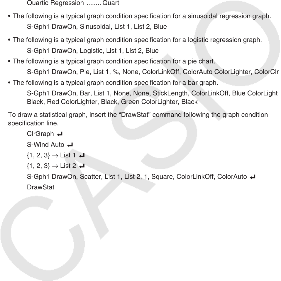
Quartic Regression ........ Quart
• The following is a typical graph condition specification for a sinusoidal regression graph.
S-Gph1 DrawOn, Sinusoidal, List 1, List 2, Blue
• The following is a typical graph condition specification for a logistic regression graph.
S-Gph1 DrawOn, Logistic, List 1, List 2, Blue
• The following is a typical graph condition specification for a pie chart.
S-Gph1 DrawOn, Pie, List 1, %, None, ColorLinkOff, ColorAuto ColorLighter, ColorClr
• The following is a typical graph condition specification for a bar graph.
S-Gph1 DrawOn, Bar, List 1, None, None, StickLength, ColorLinkOff, Blue ColorLighter,
Black, Red ColorLighter, Black, Green ColorLighter, Black
To draw a statistical graph, insert the “DrawStat” command following the graph condition
specification line.
ClrGraph _
S-Wind Auto _
{1, 2, 3} → List 1 _
{1, 2, 3} → List 2 _
S-Gph1 DrawOn, Scatter, List 1, List 2, 1, Square, ColorLinkOff, ColorAuto _
DrawStat