
User Manual
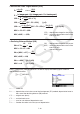
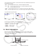
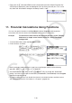
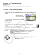
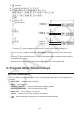
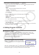

Table Of Contents
- Contents
- Getting Acquainted — Read This First!
- Chapter 1 Basic Operation
- Chapter 2 Manual Calculations
- 1. Basic Calculations
- 2. Special Functions
- 3. Specifying the Angle Unit and Display Format
- 4. Function Calculations
- 5. Numerical Calculations
- 6. Complex Number Calculations
- 7. Binary, Octal, Decimal, and Hexadecimal Calculations with Integers
- 8. Matrix Calculations
- 9. Vector Calculations
- 10. Metric Conversion Calculations
- Chapter 3 List Function
- Chapter 4 Equation Calculations
- Chapter 5 Graphing
- 1. Sample Graphs
- 2. Controlling What Appears on a Graph Screen
- 3. Drawing a Graph
- 4. Saving and Recalling Graph Screen Contents
- 5. Drawing Two Graphs on the Same Screen
- 6. Manual Graphing
- 7. Using Tables
- 8. Modifying a Graph
- 9. Dynamic Graphing
- 10. Graphing a Recursion Formula
- 11. Graphing a Conic Section
- 12. Drawing Dots, Lines, and Text on the Graph Screen (Sketch)
- 13. Function Analysis
- Chapter 6 Statistical Graphs and Calculations
- 1. Before Performing Statistical Calculations
- 2. Calculating and Graphing Single-Variable Statistical Data
- 3. Calculating and Graphing Paired-Variable Statistical Data (Curve Fitting)
- 4. Performing Statistical Calculations
- 5. Tests
- 6. Confidence Interval
- 7. Distribution
- 8. Input and Output Terms of Tests, Confidence Interval, and Distribution
- 9. Statistic Formula
- Chapter 7 Financial Calculation
- Chapter 8 Programming
- Chapter 9 Spreadsheet
- Chapter 10 eActivity
- Chapter 11 Memory Manager
- Chapter 12 System Manager
- Chapter 13 Data Communication
- Chapter 14 Geometry
- Chapter 15 Picture Plot
- Chapter 16 3D Graph Function
- Appendix
- Examination Mode
- E-CON4 Application (English)
- 1. E-CON4 Mode Overview
- 2. Sampling Screen
- 3. Auto Sensor Detection (CLAB Only)
- 4. Selecting a Sensor
- 5. Configuring the Sampling Setup
- 6. Performing Auto Sensor Calibration and Zero Adjustment
- 7. Using a Custom Probe
- 8. Using Setup Memory
- 9. Starting a Sampling Operation
- 10. Using Sample Data Memory
- 11. Using the Graph Analysis Tools to Graph Data
- 12. Graph Analysis Tool Graph Screen Operations
- 13. Calling E-CON4 Functions from an eActivity
7-16
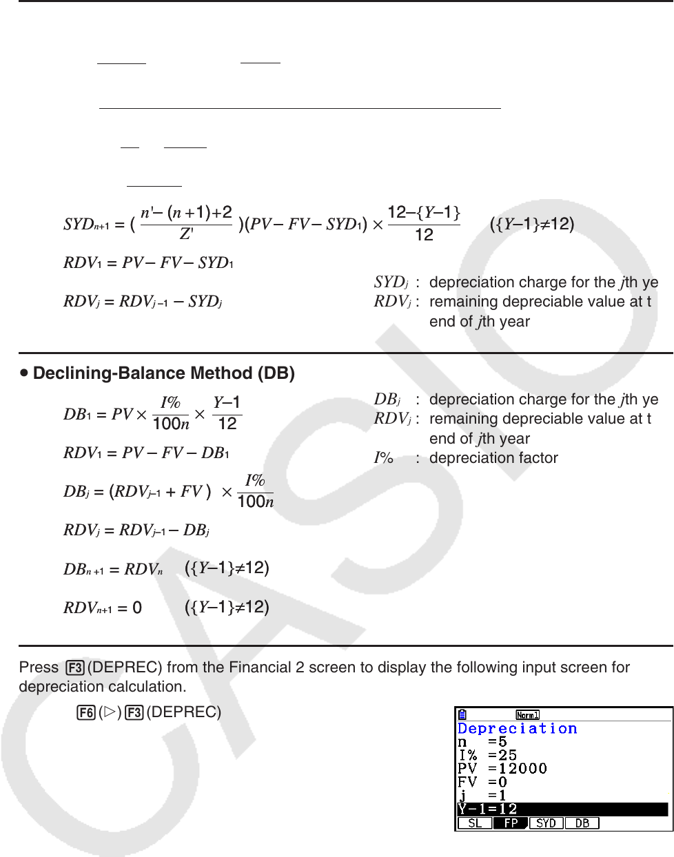
u Sum-of-the-Years’-Digits Method (SYD)
SYD j : depreciation charge for the j th year
RDV j : remaining depreciable value at the
end of
j th year
u Declining-Balance Method (DB)
DB
j : depreciation charge for the j th year
RDV j : remaining depreciable value at the
end of j th year
I % : depreciation factor
Press 3(DEPREC) from the Financial 2 screen to display the following input screen for
depreciation calculation.
6( g) 3(DEPREC)
n ............ useful life
I % ......... depreciation ratio in the case of the fixed percent (FP) method, depreciation factor in
the case of the declining balance (DB) method
P V ......... original cost (basis)
F V ......... residual book value
j ............. year for calculation of depreciation cost
Y −1 ........ number of months in the first year of depreciation
n (n +1)
Z =
2
2
(n' integer part +1)(n' integer part + 2*n' fraction part
)
Z' =
SYD
1 =
{Y–1}
12
n
Z
× (PV
– FV )
n'– j+2
Z'
)(PV
– FV – SYD1)( j≠1)SYDj = (
RDV1 = PV – FV – SYD1
RDVj = RDVj –1 – SYDj
n'– (n +1)+2
Z'
)(PV
– FV – SYD1)({Y–1}≠12)
12–{Y–1}
12
×SYD
n+1 = (
12
{Y–1}
n' = n –
n (n +1)
Z =
2
2
(n' integer part +1)(n' integer part + 2*n' fraction part
)
Z' =
SYD
1 =
{Y–1}
12
n
Z
× (PV
– FV )
n'– j+2
Z'
)(PV
– FV – SYD1)( j≠1)SYDj = (
RDV1 = PV – FV – SYD1
RDVj = RDVj –1 – SYDj
n'– (n +1)+2
Z'
)(PV
– FV – SYD1)({Y–1}≠12)
12–{Y–1}
12
×SYD
n+1 = (
12
{Y–1}
n' = n –
RDV1 = PV – FV – DB1
({Y–1}≠12)
({Y–1}≠12)
100n
Y–1I%
DB
1 = PV ×
100n
I%
12
×
×
DB
j = (RDVj–1 + FV )
RDVj = RDVj–1 – DBj
DBn +1 = RDVn
RDVn+1 = 0
RDV
1 = PV – FV – DB1
({Y–1}≠12)
({Y–1}≠12)
100n
Y–1I%
DB
1 = PV ×
100n
I%
12
×
×
DB
j = (RDVj–1 + FV )
RDVj = RDVj–1 – DBj
DBn +1 = RDVn
RDVn+1 = 0