
User Manual
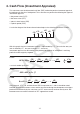
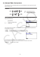


Table Of Contents
- Contents
- Getting Acquainted — Read This First!
- Chapter 1 Basic Operation
- Chapter 2 Manual Calculations
- 1. Basic Calculations
- 2. Special Functions
- 3. Specifying the Angle Unit and Display Format
- 4. Function Calculations
- 5. Numerical Calculations
- 6. Complex Number Calculations
- 7. Binary, Octal, Decimal, and Hexadecimal Calculations with Integers
- 8. Matrix Calculations
- 9. Vector Calculations
- 10. Metric Conversion Calculations
- Chapter 3 List Function
- Chapter 4 Equation Calculations
- Chapter 5 Graphing
- 1. Sample Graphs
- 2. Controlling What Appears on a Graph Screen
- 3. Drawing a Graph
- 4. Saving and Recalling Graph Screen Contents
- 5. Drawing Two Graphs on the Same Screen
- 6. Manual Graphing
- 7. Using Tables
- 8. Modifying a Graph
- 9. Dynamic Graphing
- 10. Graphing a Recursion Formula
- 11. Graphing a Conic Section
- 12. Drawing Dots, Lines, and Text on the Graph Screen (Sketch)
- 13. Function Analysis
- Chapter 6 Statistical Graphs and Calculations
- 1. Before Performing Statistical Calculations
- 2. Calculating and Graphing Single-Variable Statistical Data
- 3. Calculating and Graphing Paired-Variable Statistical Data (Curve Fitting)
- 4. Performing Statistical Calculations
- 5. Tests
- 6. Confidence Interval
- 7. Distribution
- 8. Input and Output Terms of Tests, Confidence Interval, and Distribution
- 9. Statistic Formula
- Chapter 7 Financial Calculation
- Chapter 8 Programming
- Chapter 9 Spreadsheet
- Chapter 10 eActivity
- Chapter 11 Memory Manager
- Chapter 12 System Manager
- Chapter 13 Data Communication
- Chapter 14 Geometry
- Chapter 15 Picture Plot
- Chapter 16 3D Graph Function
- Appendix
- Examination Mode
- E-CON4 Application (English)
- 1. E-CON4 Mode Overview
- 2. Sampling Screen
- 3. Auto Sensor Detection (CLAB Only)
- 4. Selecting a Sensor
- 5. Configuring the Sampling Setup
- 6. Performing Auto Sensor Calibration and Zero Adjustment
- 7. Using a Custom Probe
- 8. Using Setup Memory
- 9. Starting a Sampling Operation
- 10. Using Sample Data Memory
- 11. Using the Graph Analysis Tools to Graph Data
- 12. Graph Analysis Tool Graph Screen Operations
- 13. Calling E-CON4 Functions from an eActivity
7-7
4. Cash Flow (Investment Appraisal)
This calculator uses the discounted cash flow (DCF) method to perform investment appraisal
by totalling cash flow for a fixed period. This calculator can perform the following four types of
investment appraisal.
• Net present value (
NPV )
• Net future value (
NFV )
• Internal rate of return (
IRR )
• Payback period (
PBP )
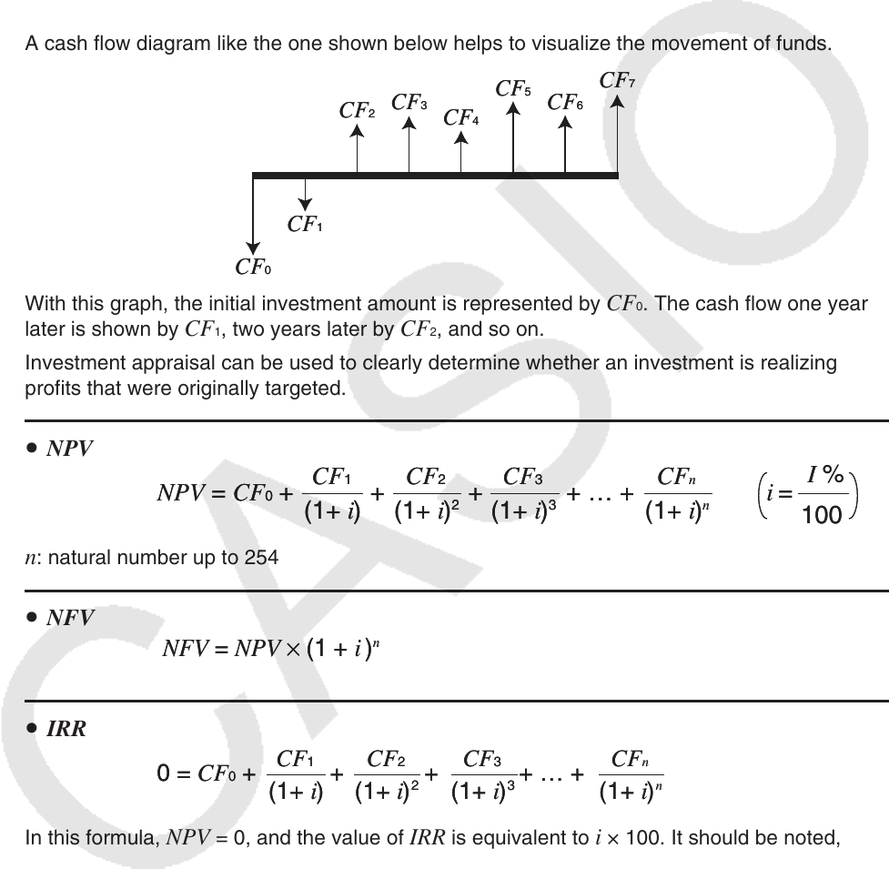
A cash flow diagram like the one shown below helps to visualize the movement of funds.
With this graph, the initial investment amount is represented by CF 0 . The cash flow one year
later is shown by CF 1 , two years later by CF 2 , and so on.
Investment appraisal can be used to clearly determine whether an investment is realizing
profits that were originally targeted.
u NPV
n : natural number up to 254
u NFV
u IRR
In this formula, NPV = 0, and the value of IRR is equivalent to i × 100. It should be noted,
however, that minute fractional values tend to accumulate during the subsequent calculations
performed automatically by the calculator, so NPV never actually reaches exactly zero. IRR
becomes more accurate the closer that NPV approaches to zero.
CF0
CF1
CF2
CF3
CF4
CF5
CF6
CF7
CF0
CF1
CF2
CF3
CF4
CF5
CF6
CF7
NPV = CF0 + + + + … +
(1+ i)
CF
1
(1+ i)
2
CF2
(1+ i)
3
CF3
(1+ i)
n
CFn
i =
100
I %
NPV = CF0 + + + + … +
(1+ i)
CF
1
(1+ i)
2
CF2
(1+ i)
3
CF3
(1+ i)
n
CFn
i =
100
I %
NFV = NPV × (1 + i )
n
NFV = NPV × (1 + i )
n
0 = CF0 + + + + … +
(1+ i)
CF
1
(1+ i)
2
CF2
(1+ i)
3
CF3
(1+ i)
n
CFn
0 = CF0 + + + + … +
(1+ i)
CF
1
(1+ i)
2
CF2
(1+ i)
3
CF3
(1+ i)
n
CFn