User Manual

ManualsBrandsCasio ManualsCalculatorsCasio fx-CG10/fx-CG20

251

252

253

254

255

256

257

258

259

260

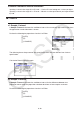
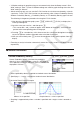
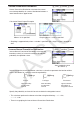
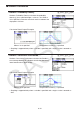
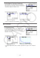
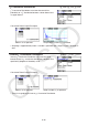
Table Of Contents

Contents
Getting Acquainted — Read This First!
Chapter 1 Basic Operation
- 1. Keys
- 2. Display
- 3. Inputting and Editing Calculations
- 4. Using the Math Input/Output Mode
- 5. Option (OPTN) Menu
- 6. Variable Data (VARS) Menu
- 7. Program (PRGM) Menu
- 8. Using the Setup Screen
- 9. Using Screen Capture
- 10. When you keep having problems...
Chapter 2 Manual Calculations
- 1. Basic Calculations
- 2. Special Functions
- 3. Specifying the Angle Unit and Display Format
- 4. Function Calculations
- 5. Numerical Calculations
- 6. Complex Number Calculations
- 7. Binary, Octal, Decimal, and Hexadecimal Calculations with Integers
- 8. Matrix Calculations
- 9. Vector Calculations
- 10. Metric Conversion Calculations
Chapter 3 List Function
- 1. Inputting and Editing a List
- 2. Manipulating List Data
- 3. Arithmetic Calculations Using Lists
- 4. Switching between List Files
- 5. Using CSV Files
Chapter 4 Equation Calculations
- 1. Simultaneous Linear Equations
- 2. High-order Equations from 2nd to 6th Degree
- 3. Solve Calculations
Chapter 5 Graphing
- 1. Sample Graphs
- 2. Controlling What Appears on a Graph Screen
- 3. Drawing a Graph
- 4. Saving and Recalling Graph Screen Contents
- 5. Drawing Two Graphs on the Same Screen
- 6. Manual Graphing
- 7. Using Tables
- 8. Modifying a Graph
- 9. Dynamic Graphing
- 10. Graphing a Recursion Formula
- 11. Graphing a Conic Section
- 12. Drawing Dots, Lines, and Text on the Graph Screen (Sketch)
- 13. Function Analysis
Chapter 6 Statistical Graphs and Calculations
- 1. Before Performing Statistical Calculations
- 2. Calculating and Graphing Single-Variable Statistical Data
- 3. Calculating and Graphing Paired-Variable Statistical Data (Curve Fitting)
- 4. Performing Statistical Calculations
- 5. Tests
- 6. Confidence Interval
- 7. Distribution
- 8. Input and Output Terms of Tests, Confidence Interval, and Distribution
- 9. Statistic Formula
Chapter 7 Financial Calculation
- 1. Before Performing Financial Calculations
- 2. Simple Interest
- 3. Compound Interest
- 4. Cash Flow (Investment Appraisal)
- 5. Amortization
- 6. Interest Rate Conversion
- 7. Cost, Selling Price, Margin
- 8. Day/Date Calculations
- 9. Depreciation
- 10. Bond Calculations
- 11. Financial Calculations Using Functions
Chapter 8 Programming
- 1. Basic Programming Steps
- 2. Program Mode Function Keys
- 3. Editing Program Contents
- 4. File Management
- 5. Command Reference
- 6. Using Calculator Functions in Programs
- 7. Program Mode Command List
- 8. CASIO Scientific Function Calculator Special Commands ‹=› Text Conversion Table
- 9. Program Library
Chapter 9 Spreadsheet
- 1. Spreadsheet Basics and the Function Menu
- 2. Basic Spreadsheet Operations
- 3. Using Special Spreadsheet Mode Commands
- 4. Conditional Formatting
- 5. Drawing Statistical Graphs, and Performing Statistical and Regression Calculations
- 6. Spreadsheet Mode Memory
Chapter 10 eActivity
- 1. eActivity Overview
- 2. eActivity Function Menus
- 3. eActivity File Operations
- 4. Inputting and Editing Data
Chapter 11 Memory Manager
- 1. Using the Memory Manager
Chapter 12 System Manager
- 1. Using the System Manager
- 2. System Settings
Chapter 13 Data Communication
- 1. Performing Data Communication between the Calculator and a Personal Computer
- 2. Performing Data Communication between Two Calculators
- 3. Connecting the Calculator to a Projector
Chapter 14 Geometry
- 1. Geometry Mode Overview
- 2. Drawing and Editing Objects
- 3. Controlling the Appearance of the Geometry Window
- 4. Using Text and Labels in a Screen Image
- 5. Using the Measurement Box
- 6. Working with Animations
Chapter 15 Picture Plot
- 1. Picture Plot Function Menus
- 2. Managing Picture Plot Files
- 3. Using the Plot Function
- 4. Using the Plot List
- 5. Common Functions with the Graph Mode
Chapter 16 3D Graph Function
- 1. Example of Drawing in the 3D Graph Mode
- 2. 3D View Window
- 3. 3D Graph Function List
- 4. 3D Graph Function Selection Screen
- 5. 3D Graph Screen
Appendix
- 1. Error Message Table
- 2. Input Ranges
Examination Mode
E-CON4 Application (English)
- 1. E-CON4 Mode Overview
- 2. Sampling Screen
- 3. Auto Sensor Detection (CLAB Only)
- 4. Selecting a Sensor
- 5. Configuring the Sampling Setup
- 6. Performing Auto Sensor Calibration and Zero Adjustment
- 7. Using a Custom Probe
- 8. Using Setup Memory
- 9. Starting a Sampling Operation
- 10. Using Sample Data Memory
- 11. Using the Graph Analysis Tools to Graph Data
- 12. Graph Analysis Tool Graph Screen Operations
- 13. Calling E-CON4 Functions from an eActivity

6-51

Normal probability density calculates the probability density of normal distribution from a

specified

x value.

Normal cumulative distribution calculates the probability of normal distribution data falling

between two specific values.

Inverse normal cumulative distribution calculates a value that represents the location within

a normal distribution for a specific cumulative probability.

Student- t probability density calculates t probability density from a specified x value.

Student- t cumulative distribution calculates the probability of t distribution data falling

between two specific values.

Inverse Student- t cumulative distribution calculates the lower bound value of a Student- t

cumulative probability density for a specified percentage.

Like t distribution, probability density (or probability), cumulative distribution and inverse

cumulative distribution can also be calculated for

, F , Binomial , Poisson , Geometric and

Hypergeometric distributions.

On the initial Statistics mode screen, press 5(DIST) to display the distribution menu, which

contains the following items.

• 5(DIST) 1(NORM) ... Normal distribution (page 6-52)

2(t) ... Student-

t distribution (page 6-54)

3(CHI) ... χ

distribution (page 6-55)

4(F) ...

F distribution (page 6-57)

5(BINOMIAL) ... Binomial distribution (page 6-58)

6( g) 1(POISSON) ... Poisson distribution (page 6-60)

6( g) 2(GEO) ... Geometric distribution (page 6-62)

6( g) 3(HYPRGEO) ... Hypergeometric distribution (page 6-64)

After setting all the parameters, use c to move the highlighting to “Execute” and then press

one of the function keys shown below to perform the calculation or draw the graph.

• 1(CALC) ... Performs the calculation.

• 6(DRAW) ... Draws the graph.

k Common Distribution Functions

• Before drawing the graph of a distribution calculation result, you can use the procedure

below to specify the graph line color (when Data:Variable only).

1. Display the distribution input screen.

• To display the normal probability density input screen, for example, display the List Editor

and then press 5(DIST)1(NORM)1(Npd).

2. Move the highlighting to “GphColor” and then press 1(COLOR).

3. On the color selection dialog box that appears, use the cursor keys to move the

highlighting to the desired color and then press w.