
User Manual
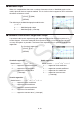
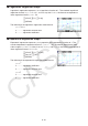
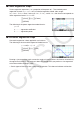

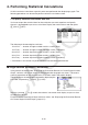
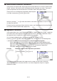

Table Of Contents
- Contents
- Getting Acquainted — Read This First!
- Chapter 1 Basic Operation
- Chapter 2 Manual Calculations
- 1. Basic Calculations
- 2. Special Functions
- 3. Specifying the Angle Unit and Display Format
- 4. Function Calculations
- 5. Numerical Calculations
- 6. Complex Number Calculations
- 7. Binary, Octal, Decimal, and Hexadecimal Calculations with Integers
- 8. Matrix Calculations
- 9. Vector Calculations
- 10. Metric Conversion Calculations
- Chapter 3 List Function
- Chapter 4 Equation Calculations
- Chapter 5 Graphing
- 1. Sample Graphs
- 2. Controlling What Appears on a Graph Screen
- 3. Drawing a Graph
- 4. Saving and Recalling Graph Screen Contents
- 5. Drawing Two Graphs on the Same Screen
- 6. Manual Graphing
- 7. Using Tables
- 8. Modifying a Graph
- 9. Dynamic Graphing
- 10. Graphing a Recursion Formula
- 11. Graphing a Conic Section
- 12. Drawing Dots, Lines, and Text on the Graph Screen (Sketch)
- 13. Function Analysis
- Chapter 6 Statistical Graphs and Calculations
- 1. Before Performing Statistical Calculations
- 2. Calculating and Graphing Single-Variable Statistical Data
- 3. Calculating and Graphing Paired-Variable Statistical Data (Curve Fitting)
- 4. Performing Statistical Calculations
- 5. Tests
- 6. Confidence Interval
- 7. Distribution
- 8. Input and Output Terms of Tests, Confidence Interval, and Distribution
- 9. Statistic Formula
- Chapter 7 Financial Calculation
- Chapter 8 Programming
- Chapter 9 Spreadsheet
- Chapter 10 eActivity
- Chapter 11 Memory Manager
- Chapter 12 System Manager
- Chapter 13 Data Communication
- Chapter 14 Geometry
- Chapter 15 Picture Plot
- Chapter 16 3D Graph Function
- Appendix
- Examination Mode
- E-CON4 Application (English)
- 1. E-CON4 Mode Overview
- 2. Sampling Screen
- 3. Auto Sensor Detection (CLAB Only)
- 4. Selecting a Sensor
- 5. Configuring the Sampling Setup
- 6. Performing Auto Sensor Calibration and Zero Adjustment
- 7. Using a Custom Probe
- 8. Using Setup Memory
- 9. Starting a Sampling Operation
- 10. Using Sample Data Memory
- 11. Using the Graph Analysis Tools to Graph Data
- 12. Graph Analysis Tool Graph Screen Operations
- 13. Calling E-CON4 Functions from an eActivity
6-25
u Calculation of the Correlation Coefficient (r), Coefficient of Determination
(r
2
) and Mean Square Error (MSe)
After the regression formula parameters on the regression calculation result screen, the
following parameters also appear on the display. The parameters that appear depend on the
regression formula.
Correlation coefficient (r)
Displayed following: linear regression, logarithmic regression, exponential regression, or power
regression calculation.
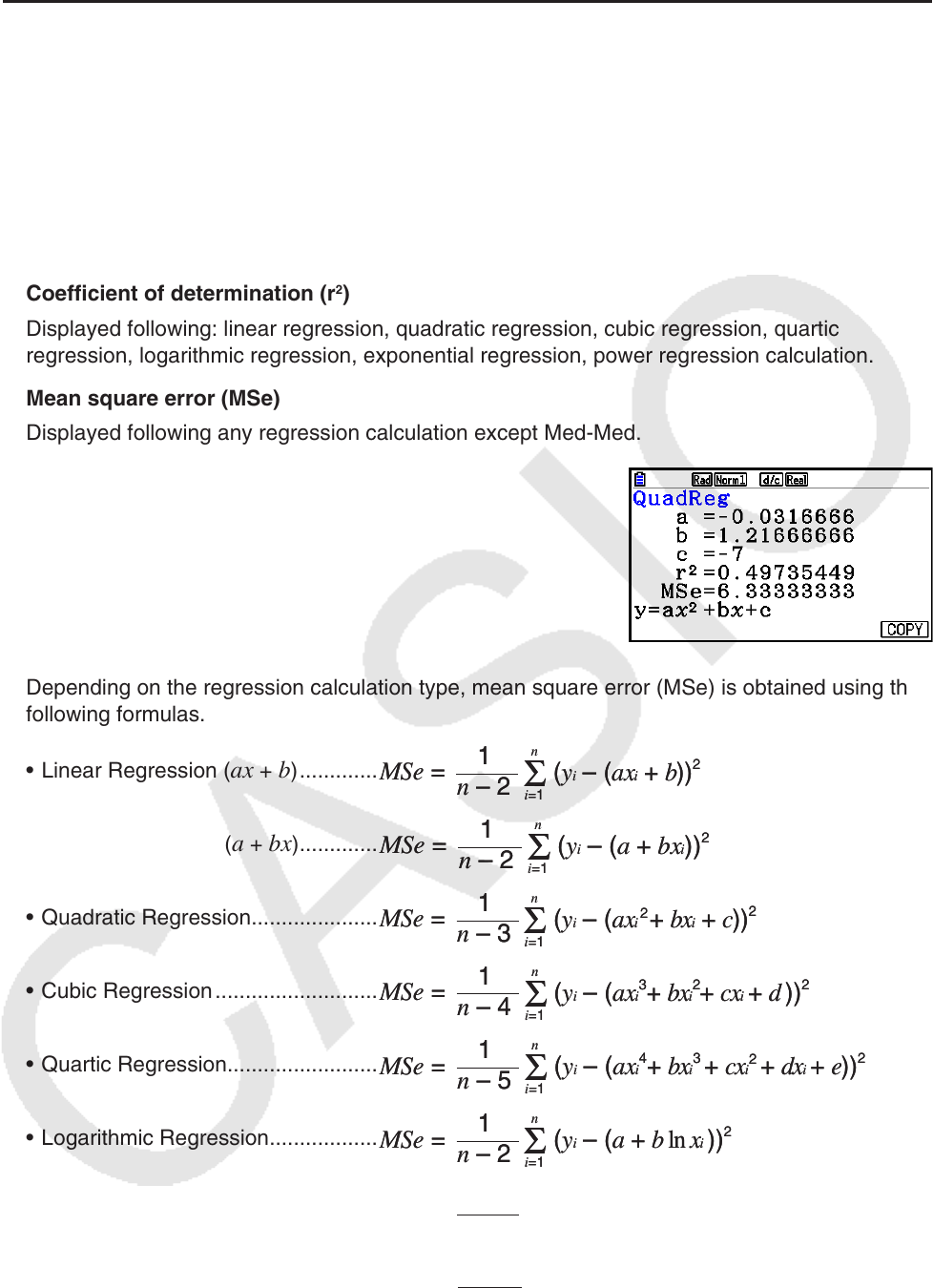
Coefficient of determination (r
2
)
Displayed following: linear regression, quadratic regression, cubic regression, quartic
regression, logarithmic regression, exponential regression, power regression calculation.
Mean square error (MSe)
Displayed following any regression calculation except Med-Med.
Depending on the regression calculation type, mean square error (MSe) is obtained using the
following formulas.
• Linear Regression (
ax + b ) .............
(
a + bx ) .............
• Quadratic Regression .....................
• Cubic Regression ...........................
• Quartic Regression .........................
• Logarithmic Regression ..................
• Exponential Regression (
a · e
bx
) .......
(
a · b
x
) ........
M
Se =
Σ
1
n – 2
i=1
n
(y
i
– (ax
i
+ b))
2
M
Se =
Σ
1
n – 2
i=1
n
(y
i
– (ax
i
+ b))
2
M
Se =
Σ
1
n – 2
i=1
n
(yi – (a + bxi))
2
M
Se =
Σ
1
n – 2
i=1
n
(yi – (a + bxi))
2
M
Se =
Σ
1
n – 3
i=1
n
(y
i
– (ax
i
+ bx
i
+ c))
2
2
M
Se =
Σ
1
n – 3
i=1
n
(y
i
– (ax
i
+ bx
i
+ c))
2
2
M
Se =
Σ
1
n – 4
i=1
n
(y
i
– (ax
i
3
+ bx
i
+ cx
i
+ d ))
2
2
M
Se =
Σ
1
n – 4
i=1
n
(y
i
– (ax
i
3
+ bx
i
+ cx
i
+ d ))
2
2
M
Se =
Σ
1
n – 5
i=1
n
(yi – (axi
4
+ bxi
3
+ cxi
+ dxi
+ e))
2
2
M
Se =
Σ
1
n – 5
i=1
n
(yi – (axi
4
+ bxi
3
+ cxi
+ dxi
+ e))
2
2
M
Se =
Σ
1
n – 2
i=1
n
(y
i
– (a + b ln x
i
))
2
M
Se =
Σ
1
n – 2
i=1
n
(y
i
– (a + b ln x
i
))
2
M
Se =
Σ
1
n – 2
i=1
n
(ln y
i
– (ln a + bx
i
))
2
M
Se =
Σ
1
n – 2
i=1
n
(ln y
i
– (ln a + bx
i
))
2
M
Se =
Σ
1
n – 2
i=1
n
(ln yi – (ln a + (ln b) · xi ))
2
M
Se =
Σ
1
n – 2
i=1
n
(ln yi – (ln a + (ln b) · xi ))
2