
User Manual
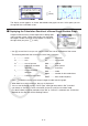
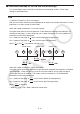
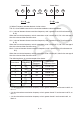
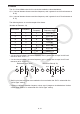
Table Of Contents
- Contents
- Getting Acquainted — Read This First!
- Chapter 1 Basic Operation
- Chapter 2 Manual Calculations
- 1. Basic Calculations
- 2. Special Functions
- 3. Specifying the Angle Unit and Display Format
- 4. Function Calculations
- 5. Numerical Calculations
- 6. Complex Number Calculations
- 7. Binary, Octal, Decimal, and Hexadecimal Calculations with Integers
- 8. Matrix Calculations
- 9. Vector Calculations
- 10. Metric Conversion Calculations
- Chapter 3 List Function
- Chapter 4 Equation Calculations
- Chapter 5 Graphing
- 1. Sample Graphs
- 2. Controlling What Appears on a Graph Screen
- 3. Drawing a Graph
- 4. Saving and Recalling Graph Screen Contents
- 5. Drawing Two Graphs on the Same Screen
- 6. Manual Graphing
- 7. Using Tables
- 8. Modifying a Graph
- 9. Dynamic Graphing
- 10. Graphing a Recursion Formula
- 11. Graphing a Conic Section
- 12. Drawing Dots, Lines, and Text on the Graph Screen (Sketch)
- 13. Function Analysis
- Chapter 6 Statistical Graphs and Calculations
- 1. Before Performing Statistical Calculations
- 2. Calculating and Graphing Single-Variable Statistical Data
- 3. Calculating and Graphing Paired-Variable Statistical Data (Curve Fitting)
- 4. Performing Statistical Calculations
- 5. Tests
- 6. Confidence Interval
- 7. Distribution
- 8. Input and Output Terms of Tests, Confidence Interval, and Distribution
- 9. Statistic Formula
- Chapter 7 Financial Calculation
- Chapter 8 Programming
- Chapter 9 Spreadsheet
- Chapter 10 eActivity
- Chapter 11 Memory Manager
- Chapter 12 System Manager
- Chapter 13 Data Communication
- Chapter 14 Geometry
- Chapter 15 Picture Plot
- Chapter 16 3D Graph Function
- Appendix
- Examination Mode
- E-CON4 Application (English)
- 1. E-CON4 Mode Overview
- 2. Sampling Screen
- 3. Auto Sensor Detection (CLAB Only)
- 4. Selecting a Sensor
- 5. Configuring the Sampling Setup
- 6. Performing Auto Sensor Calibration and Zero Adjustment
- 7. Using a Custom Probe
- 8. Using Setup Memory
- 9. Starting a Sampling Operation
- 10. Using Sample Data Memory
- 11. Using the Graph Analysis Tools to Graph Data
- 12. Graph Analysis Tool Graph Screen Operations
- 13. Calling E-CON4 Functions from an eActivity
6-17
k Displaying Regression Calculation Results
Whenever you perform a regression calculation, the regression formula parameter (such
as a and b in the linear regression y = ax + b ) calculation results appear on the display. The
regression formula parameter calculation results also appear as soon as you press 1(CALC)
and then a function key to select a regression type, while a graph is on the display.
The following parameters will also appear on the regression calculation result screen.
r ..............correlation coefficient (linear regression, logarithmic regression, exponential
regression, and power regression only)
r
2
.............coefficient of determination (except for Med-Med, sinusoidal regression, and
logistic regression)
MSe .........mean square error (except for Med-Med)
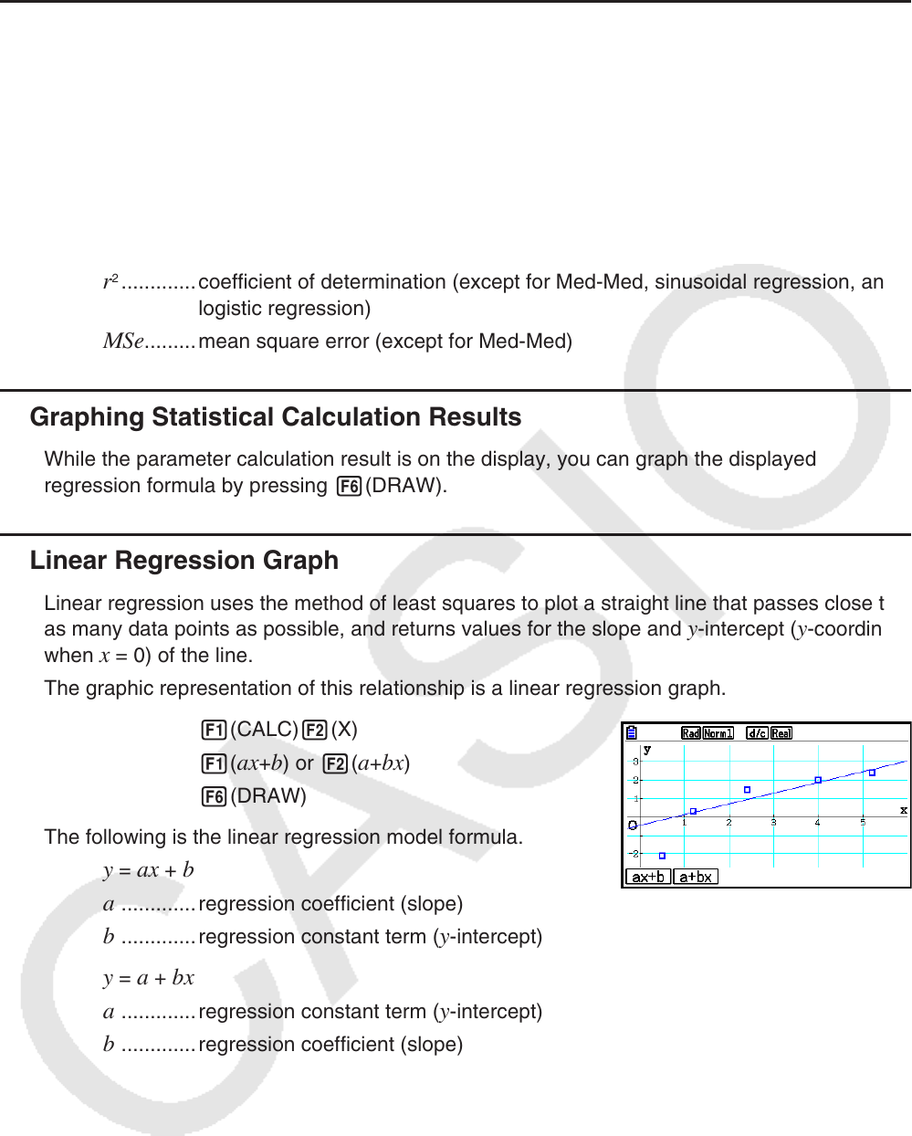
k Graphing Statistical Calculation Results
While the parameter calculation result is on the display, you can graph the displayed
regression formula by pressing 6(DRAW).
k Linear Regression Graph
Linear regression uses the method of least squares to plot a straight line that passes close to
as many data points as possible, and returns values for the slope and y -intercept ( y -coordinate
when x = 0) of the line.
The graphic representation of this relationship is a linear regression graph.
1(CALC) 2(X)
1(
ax + b ) or 2( a + bx )
6(DRAW)
The following is the linear regression model formula.
y = ax + b
a
.............regression coefficient (slope)
b .............regression constant term ( y -intercept)
y = a + bx
a
.............regression constant term ( y -intercept)
b .............regression coefficient (slope)