
User Manual
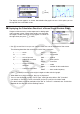
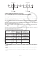
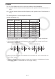
Table Of Contents
- Contents
- Getting Acquainted — Read This First!
- Chapter 1 Basic Operation
- Chapter 2 Manual Calculations
- 1. Basic Calculations
- 2. Special Functions
- 3. Specifying the Angle Unit and Display Format
- 4. Function Calculations
- 5. Numerical Calculations
- 6. Complex Number Calculations
- 7. Binary, Octal, Decimal, and Hexadecimal Calculations with Integers
- 8. Matrix Calculations
- 9. Vector Calculations
- 10. Metric Conversion Calculations
- Chapter 3 List Function
- Chapter 4 Equation Calculations
- Chapter 5 Graphing
- 1. Sample Graphs
- 2. Controlling What Appears on a Graph Screen
- 3. Drawing a Graph
- 4. Saving and Recalling Graph Screen Contents
- 5. Drawing Two Graphs on the Same Screen
- 6. Manual Graphing
- 7. Using Tables
- 8. Modifying a Graph
- 9. Dynamic Graphing
- 10. Graphing a Recursion Formula
- 11. Graphing a Conic Section
- 12. Drawing Dots, Lines, and Text on the Graph Screen (Sketch)
- 13. Function Analysis
- Chapter 6 Statistical Graphs and Calculations
- 1. Before Performing Statistical Calculations
- 2. Calculating and Graphing Single-Variable Statistical Data
- 3. Calculating and Graphing Paired-Variable Statistical Data (Curve Fitting)
- 4. Performing Statistical Calculations
- 5. Tests
- 6. Confidence Interval
- 7. Distribution
- 8. Input and Output Terms of Tests, Confidence Interval, and Distribution
- 9. Statistic Formula
- Chapter 7 Financial Calculation
- Chapter 8 Programming
- Chapter 9 Spreadsheet
- Chapter 10 eActivity
- Chapter 11 Memory Manager
- Chapter 12 System Manager
- Chapter 13 Data Communication
- Chapter 14 Geometry
- Chapter 15 Picture Plot
- Chapter 16 3D Graph Function
- Appendix
- Examination Mode
- E-CON4 Application (English)
- 1. E-CON4 Mode Overview
- 2. Sampling Screen
- 3. Auto Sensor Detection (CLAB Only)
- 4. Selecting a Sensor
- 5. Configuring the Sampling Setup
- 6. Performing Auto Sensor Calibration and Zero Adjustment
- 7. Using a Custom Probe
- 8. Using Setup Memory
- 9. Starting a Sampling Operation
- 10. Using Sample Data Memory
- 11. Using the Graph Analysis Tools to Graph Data
- 12. Graph Analysis Tool Graph Screen Operations
- 13. Calling E-CON4 Functions from an eActivity
6-14
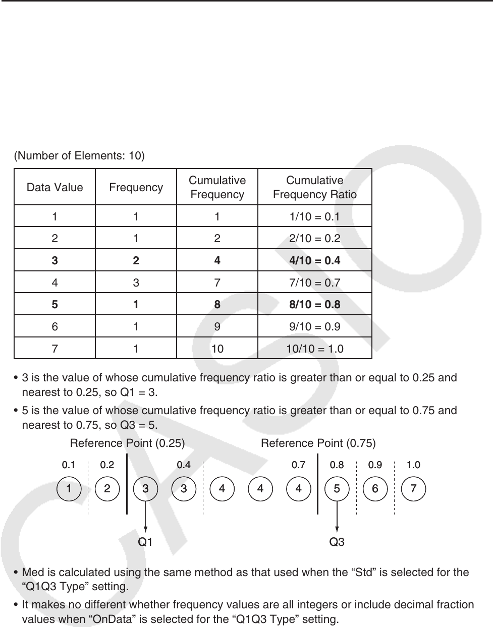
u OnData
The Q1, Q3 and Med values for this calculation method are described below.
Q1 = {value of element whose cumulative frequency ratio is greater than 0.25 and nearest to
0.25}
Q3 = {value of element whose cumulative frequency ratio is greater than 0.75 and nearest to
0.75}
The following shows an actual example of the above.
(Number of Elements: 10)
Data Value Frequency
Cumulative
Frequency
Cumulative
Frequency Ratio
1 1 1 1/10 = 0.1
2 1 2 2/10 = 0.2
3 2 4 4/10 = 0.4
4 3 7 7/10 = 0.7
5 1 8 8/10 = 0.8
6 1 9 9/10 = 0.9
7 1 10 10/10 = 1.0
• 3 is the value of whose cumulative frequency ratio is greater than or equal to 0.25 and
nearest to 0.25, so Q1 = 3.
• 5 is the value of whose cumulative frequency ratio is greater than or equal to 0.75 and
nearest to 0.75, so Q3 = 5.
Reference Point (0.25) Reference Point (0.75)
• Med is calculated using the same method as that used when the “Std” is selected for the
“Q1Q3 Type” setting.
• It makes no different whether frequency values are all integers or include decimal fraction
values when “OnData” is selected for the “Q1Q3 Type” setting.
Q1
0.1 0.2 0.4 0.7 0.8 0.9 1.0
Q3
1
2633444 75
Q1
0.1 0.2 0.4 0.7 0.8 0.9 1.0
Q3
1
2633444 75