
User Manual
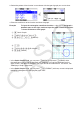
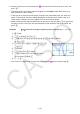
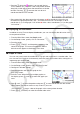
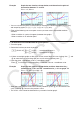
Table Of Contents
- Contents
- Getting Acquainted — Read This First!
- Chapter 1 Basic Operation
- Chapter 2 Manual Calculations
- 1. Basic Calculations
- 2. Special Functions
- 3. Specifying the Angle Unit and Display Format
- 4. Function Calculations
- 5. Numerical Calculations
- 6. Complex Number Calculations
- 7. Binary, Octal, Decimal, and Hexadecimal Calculations with Integers
- 8. Matrix Calculations
- 9. Vector Calculations
- 10. Metric Conversion Calculations
- Chapter 3 List Function
- Chapter 4 Equation Calculations
- Chapter 5 Graphing
- 1. Sample Graphs
- 2. Controlling What Appears on a Graph Screen
- 3. Drawing a Graph
- 4. Saving and Recalling Graph Screen Contents
- 5. Drawing Two Graphs on the Same Screen
- 6. Manual Graphing
- 7. Using Tables
- 8. Modifying a Graph
- 9. Dynamic Graphing
- 10. Graphing a Recursion Formula
- 11. Graphing a Conic Section
- 12. Drawing Dots, Lines, and Text on the Graph Screen (Sketch)
- 13. Function Analysis
- Chapter 6 Statistical Graphs and Calculations
- 1. Before Performing Statistical Calculations
- 2. Calculating and Graphing Single-Variable Statistical Data
- 3. Calculating and Graphing Paired-Variable Statistical Data (Curve Fitting)
- 4. Performing Statistical Calculations
- 5. Tests
- 6. Confidence Interval
- 7. Distribution
- 8. Input and Output Terms of Tests, Confidence Interval, and Distribution
- 9. Statistic Formula
- Chapter 7 Financial Calculation
- Chapter 8 Programming
- Chapter 9 Spreadsheet
- Chapter 10 eActivity
- Chapter 11 Memory Manager
- Chapter 12 System Manager
- Chapter 13 Data Communication
- Chapter 14 Geometry
- Chapter 15 Picture Plot
- Chapter 16 3D Graph Function
- Appendix
- Examination Mode
- E-CON4 Application (English)
- 1. E-CON4 Mode Overview
- 2. Sampling Screen
- 3. Auto Sensor Detection (CLAB Only)
- 4. Selecting a Sensor
- 5. Configuring the Sampling Setup
- 6. Performing Auto Sensor Calibration and Zero Adjustment
- 7. Using a Custom Probe
- 8. Using Setup Memory
- 9. Starting a Sampling Operation
- 10. Using Sample Data Memory
- 11. Using the Graph Analysis Tools to Graph Data
- 12. Graph Analysis Tool Graph Screen Operations
- 13. Calling E-CON4 Functions from an eActivity
5-58
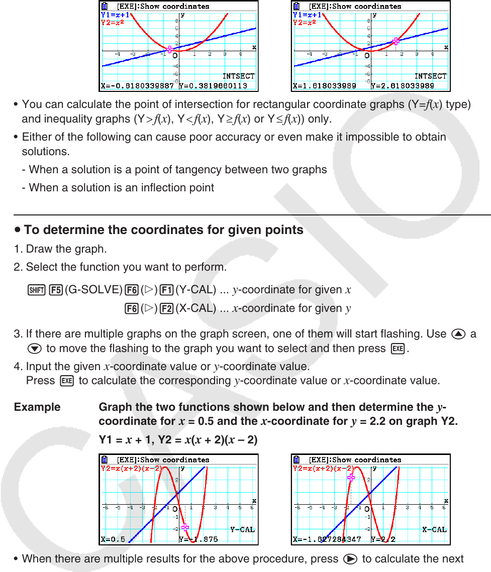
Example Graph the two functions shown below, and determine the point of
intersection between Y1 and Y2.
Y1 =
x + 1, Y2 = x
2
• You can calculate the point of intersection for rectangular coordinate graphs (Y=
f ( x ) type)
and inequality graphs (Y > f(x), Y < f(x), Y ≥ f(x) or Y ≤ f(x)) only.
• Either of the following can cause poor accuracy or even make it impossible to obtain
solutions.
- When a solution is a point of tangency between two graphs
- When a solution is an inflection point
u To determine the coordinates for given points
1. Draw the graph.
2. Select the function you want to perform.
!5(G-SOLVE) 6(g)1(Y-CAL) ...
y-coordinate for given x
6(g)2(X-CAL) ... x-coordinate for given y
3. If there are multiple graphs on the graph screen, one of them will start flashing. Use f and
c to move the flashing to the graph you want to select and then press w.
4. Input the given
x-coordinate value or y-coordinate value.
Press w to calculate the corresponding y-coordinate value or x-coordinate value.
Example Graph the two functions shown below and then determine the
y -
coordinate for x = 0.5 and the x -coordinate for y = 2.2 on graph Y2.
Y1 =
x + 1, Y2 = x ( x + 2)( x – 2)
• When there are multiple results for the above procedure, press e to calculate the next
value. Pressing d returns to the previous value.
• The X-CAL value cannot be obtained for a parametric function graph.