
User Manual
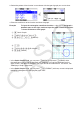
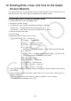
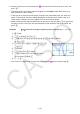
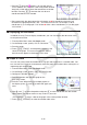
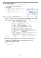
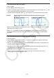
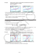
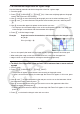
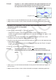
Table Of Contents
- Contents
- Getting Acquainted — Read This First!
- Chapter 1 Basic Operation
- Chapter 2 Manual Calculations
- 1. Basic Calculations
- 2. Special Functions
- 3. Specifying the Angle Unit and Display Format
- 4. Function Calculations
- 5. Numerical Calculations
- 6. Complex Number Calculations
- 7. Binary, Octal, Decimal, and Hexadecimal Calculations with Integers
- 8. Matrix Calculations
- 9. Vector Calculations
- 10. Metric Conversion Calculations
- Chapter 3 List Function
- Chapter 4 Equation Calculations
- Chapter 5 Graphing
- 1. Sample Graphs
- 2. Controlling What Appears on a Graph Screen
- 3. Drawing a Graph
- 4. Saving and Recalling Graph Screen Contents
- 5. Drawing Two Graphs on the Same Screen
- 6. Manual Graphing
- 7. Using Tables
- 8. Modifying a Graph
- 9. Dynamic Graphing
- 10. Graphing a Recursion Formula
- 11. Graphing a Conic Section
- 12. Drawing Dots, Lines, and Text on the Graph Screen (Sketch)
- 13. Function Analysis
- Chapter 6 Statistical Graphs and Calculations
- 1. Before Performing Statistical Calculations
- 2. Calculating and Graphing Single-Variable Statistical Data
- 3. Calculating and Graphing Paired-Variable Statistical Data (Curve Fitting)
- 4. Performing Statistical Calculations
- 5. Tests
- 6. Confidence Interval
- 7. Distribution
- 8. Input and Output Terms of Tests, Confidence Interval, and Distribution
- 9. Statistic Formula
- Chapter 7 Financial Calculation
- Chapter 8 Programming
- Chapter 9 Spreadsheet
- Chapter 10 eActivity
- Chapter 11 Memory Manager
- Chapter 12 System Manager
- Chapter 13 Data Communication
- Chapter 14 Geometry
- Chapter 15 Picture Plot
- Chapter 16 3D Graph Function
- Appendix
- Examination Mode
- E-CON4 Application (English)
- 1. E-CON4 Mode Overview
- 2. Sampling Screen
- 3. Auto Sensor Detection (CLAB Only)
- 4. Selecting a Sensor
- 5. Configuring the Sampling Setup
- 6. Performing Auto Sensor Calibration and Zero Adjustment
- 7. Using a Custom Probe
- 8. Using Setup Memory
- 9. Starting a Sampling Operation
- 10. Using Sample Data Memory
- 11. Using the Graph Analysis Tools to Graph Data
- 12. Graph Analysis Tool Graph Screen Operations
- 13. Calling E-CON4 Functions from an eActivity
5-55
• Pressing w while the pointer is on a graph (during
Trace, G-Solve, etc.) will place a dot at the pointer location
along with a label which shows the coordinates at the dot
location. Pressing aD removes the last dot and
coordinate label that was created.
• Dots created with the above operation will appear as
for coordinate values that are
included in the graph expression, and for values that are not. For example, a dot at
coordinates (2,1) on the graph Y=2X will be , while a dot at coordinates (2,1) on the graph
Y>2X will be
.
k Displaying the Derivative
In addition to using Trace to display coordinates, you can also display the derivative at the
current pointer location.
1. From the Main Menu, enter the Graph mode.
2. On the Setup screen, specify “On” for “Derivative”.
3. Draw the graph.
4. Press !1(TRACE), and the pointer appears at the
center of the graph. The current coordinates and the
derivative also appear on the display at this time.
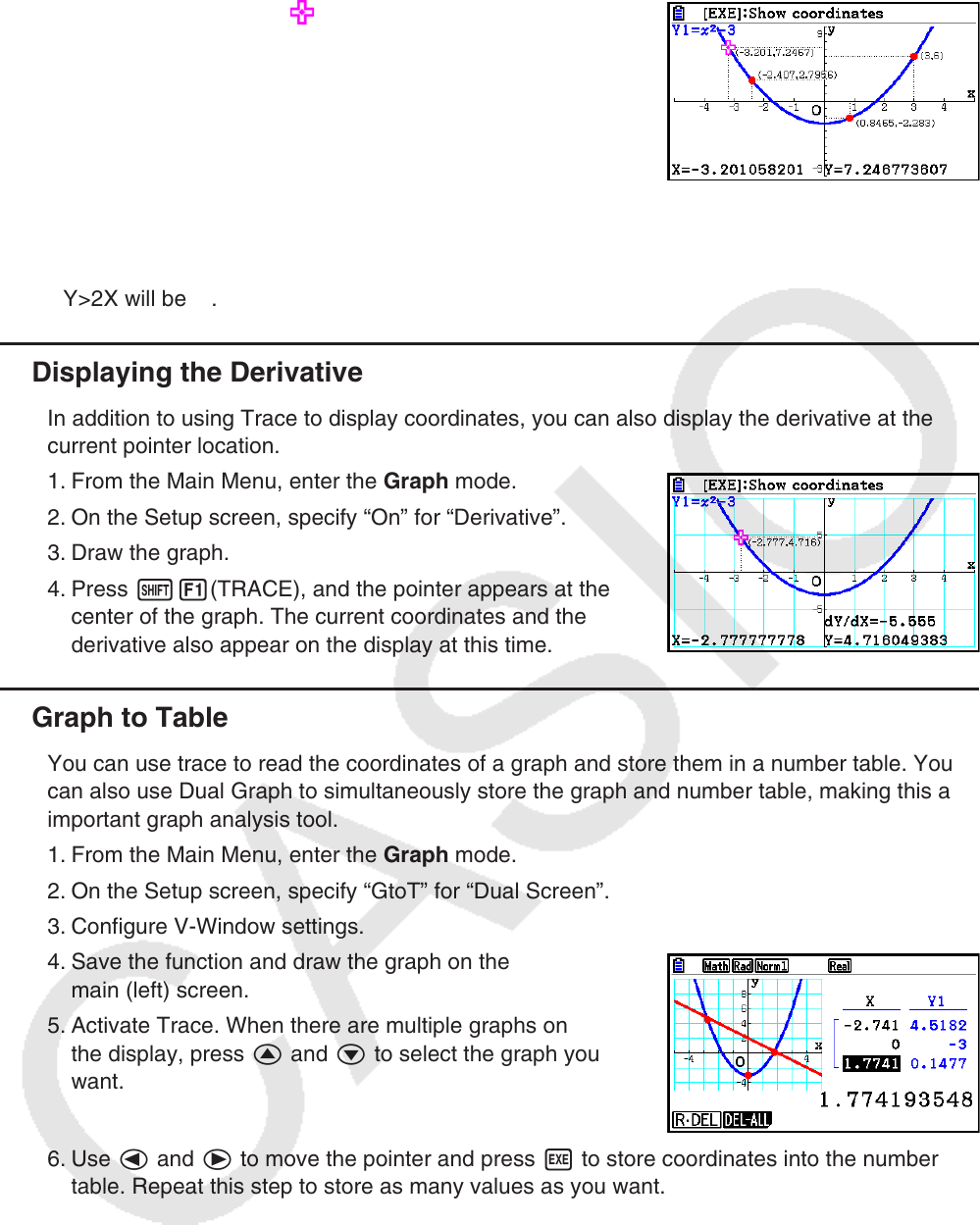
k Graph to Table
You can use trace to read the coordinates of a graph and store them in a number table. You
can also use Dual Graph to simultaneously store the graph and number table, making this an
important graph analysis tool.
1. From the Main Menu, enter the Graph mode.
2. On the Setup screen, specify “GtoT” for “Dual Screen”.
3. Configure V-Window settings.
4. Save the function and draw the graph on the
main (left) screen.
5. Activate Trace. When there are multiple graphs on
the display, press f and c to select the graph you
want.
6. Use d and e to move the pointer and press w to store coordinates into the number
table. Repeat this step to store as many values as you want.
• Each press of w places a dot on the graph at the current pointer location.
7. Press K1(CHANGE) to make the number table active.