
User Manual
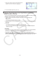
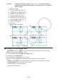
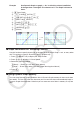
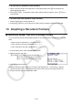
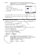
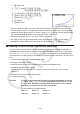
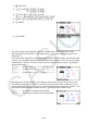
Table Of Contents
- Contents
- Getting Acquainted — Read This First!
- Chapter 1 Basic Operation
- Chapter 2 Manual Calculations
- 1. Basic Calculations
- 2. Special Functions
- 3. Specifying the Angle Unit and Display Format
- 4. Function Calculations
- 5. Numerical Calculations
- 6. Complex Number Calculations
- 7. Binary, Octal, Decimal, and Hexadecimal Calculations with Integers
- 8. Matrix Calculations
- 9. Vector Calculations
- 10. Metric Conversion Calculations
- Chapter 3 List Function
- Chapter 4 Equation Calculations
- Chapter 5 Graphing
- 1. Sample Graphs
- 2. Controlling What Appears on a Graph Screen
- 3. Drawing a Graph
- 4. Saving and Recalling Graph Screen Contents
- 5. Drawing Two Graphs on the Same Screen
- 6. Manual Graphing
- 7. Using Tables
- 8. Modifying a Graph
- 9. Dynamic Graphing
- 10. Graphing a Recursion Formula
- 11. Graphing a Conic Section
- 12. Drawing Dots, Lines, and Text on the Graph Screen (Sketch)
- 13. Function Analysis
- Chapter 6 Statistical Graphs and Calculations
- 1. Before Performing Statistical Calculations
- 2. Calculating and Graphing Single-Variable Statistical Data
- 3. Calculating and Graphing Paired-Variable Statistical Data (Curve Fitting)
- 4. Performing Statistical Calculations
- 5. Tests
- 6. Confidence Interval
- 7. Distribution
- 8. Input and Output Terms of Tests, Confidence Interval, and Distribution
- 9. Statistic Formula
- Chapter 7 Financial Calculation
- Chapter 8 Programming
- Chapter 9 Spreadsheet
- Chapter 10 eActivity
- Chapter 11 Memory Manager
- Chapter 12 System Manager
- Chapter 13 Data Communication
- Chapter 14 Geometry
- Chapter 15 Picture Plot
- Chapter 16 3D Graph Function
- Appendix
- Examination Mode
- E-CON4 Application (English)
- 1. E-CON4 Mode Overview
- 2. Sampling Screen
- 3. Auto Sensor Detection (CLAB Only)
- 4. Selecting a Sensor
- 5. Configuring the Sampling Setup
- 6. Performing Auto Sensor Calibration and Zero Adjustment
- 7. Using a Custom Probe
- 8. Using Setup Memory
- 9. Starting a Sampling Operation
- 10. Using Sample Data Memory
- 11. Using the Graph Analysis Tools to Graph Data
- 12. Graph Analysis Tool Graph Screen Operations
- 13. Calling E-CON4 Functions from an eActivity
5-50
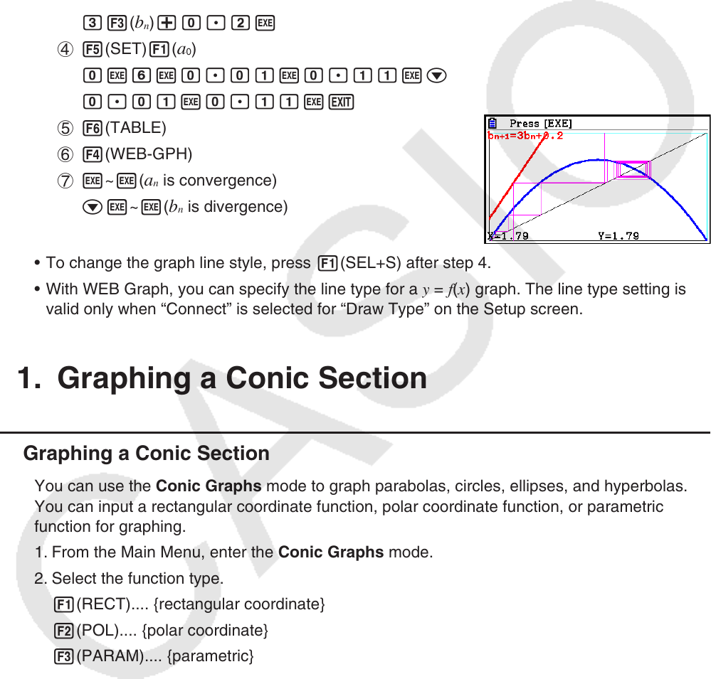
Example To draw the WEB graph for the recursion formula a
n
+1
= –3( a
n
)
2
+ 3 a
n
, b
n
+1
= 3 b
n
+ 0.2, and check for divergence or convergence. Use the following
table range: Start = 0, End = 6,
a
0
= 0.01, a
n
Str = 0.01, b
0
= 0.11, b
n
Str
= 0.11
1 m Recursion
2 !3(V-WIN) awbwbwc
awbwbwJ
3 3(TYPE) 2(
a
n
+1
) -d2( a
n
) x+d2( a
n
) w
d3(
b
n
) +a.cw
4 5(SET) 1(
a
0
)
awgwa.abwa.bbwc
a.abwa.bbwJ
5 6(TABLE)
6 4(WEB-GPH)
7 w~ w(
a
n
is convergence)
cw~w(
b
n
is divergence)
• To change the graph line style, press 1(SEL+S) after step 4.
• With WEB Graph, you can specify the line type for a y = f ( x ) graph. The line type setting is
valid only when “Connect” is selected for “Draw Type” on the Setup screen.
11. Graphing a Conic Section
k Graphing a Conic Section
You can use the Conic Graphs mode to graph parabolas, circles, ellipses, and hyperbolas.
You can input a rectangular coordinate function, polar coordinate function, or parametric
function for graphing.
1. From the Main Menu, enter the Conic Graphs mode.
2. Select the function type.
1(RECT).... {rectangular coordinate}
2(POL).... {polar coordinate}
3(PARAM).... {parametric}