
User Manual

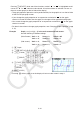
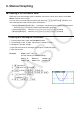
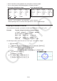
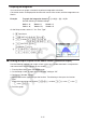
Table Of Contents
- Contents
- Getting Acquainted — Read This First!
- Chapter 1 Basic Operation
- Chapter 2 Manual Calculations
- 1. Basic Calculations
- 2. Special Functions
- 3. Specifying the Angle Unit and Display Format
- 4. Function Calculations
- 5. Numerical Calculations
- 6. Complex Number Calculations
- 7. Binary, Octal, Decimal, and Hexadecimal Calculations with Integers
- 8. Matrix Calculations
- 9. Vector Calculations
- 10. Metric Conversion Calculations
- Chapter 3 List Function
- Chapter 4 Equation Calculations
- Chapter 5 Graphing
- 1. Sample Graphs
- 2. Controlling What Appears on a Graph Screen
- 3. Drawing a Graph
- 4. Saving and Recalling Graph Screen Contents
- 5. Drawing Two Graphs on the Same Screen
- 6. Manual Graphing
- 7. Using Tables
- 8. Modifying a Graph
- 9. Dynamic Graphing
- 10. Graphing a Recursion Formula
- 11. Graphing a Conic Section
- 12. Drawing Dots, Lines, and Text on the Graph Screen (Sketch)
- 13. Function Analysis
- Chapter 6 Statistical Graphs and Calculations
- 1. Before Performing Statistical Calculations
- 2. Calculating and Graphing Single-Variable Statistical Data
- 3. Calculating and Graphing Paired-Variable Statistical Data (Curve Fitting)
- 4. Performing Statistical Calculations
- 5. Tests
- 6. Confidence Interval
- 7. Distribution
- 8. Input and Output Terms of Tests, Confidence Interval, and Distribution
- 9. Statistic Formula
- Chapter 7 Financial Calculation
- Chapter 8 Programming
- Chapter 9 Spreadsheet
- Chapter 10 eActivity
- Chapter 11 Memory Manager
- Chapter 12 System Manager
- Chapter 13 Data Communication
- Chapter 14 Geometry
- Chapter 15 Picture Plot
- Chapter 16 3D Graph Function
- Appendix
- Examination Mode
- E-CON4 Application (English)
- 1. E-CON4 Mode Overview
- 2. Sampling Screen
- 3. Auto Sensor Detection (CLAB Only)
- 4. Selecting a Sensor
- 5. Configuring the Sampling Setup
- 6. Performing Auto Sensor Calibration and Zero Adjustment
- 7. Using a Custom Probe
- 8. Using Setup Memory
- 9. Starting a Sampling Operation
- 10. Using Sample Data Memory
- 11. Using the Graph Analysis Tools to Graph Data
- 12. Graph Analysis Tool Graph Screen Operations
- 13. Calling E-CON4 Functions from an eActivity
5-26
• Certain functions can be graphed easily using built-in function graphs.
• You can draw graphs of the following built-in scientific functions.
Rectangular Coordinate Graph Polar Coordinate Graph
• sin x • cos x • tan x • sin
–1
x
• cos
–1
x • tan
–1
x • sinh x • cosh x
• tanh x • sinh
–1
x • cosh
–1
x • tanh
–1
x
• 'x • x
2
• log x • lnx
• 10
x
• e
x
• x
–1
•
3
'x
• • •
• sin
θ
• cos
θ
• tan
θ
• sin
–1
θ
• cos
–1
θ
• tan
–1
θ
• sinh
θ
• cosh
θ
• tanh
θ
• sinh
–1
θ
• cosh
–1
θ
• tanh
–1
θ
• '
θ
•
θ
2
• log
θ
• ln
θ
• 10
θ
• e
θ
•
θ
–1
•
3
'
θ
- Input for x and
θ
variables is not required for a built-in function.
- When inputting a built-in function, other operators or values cannot be input.
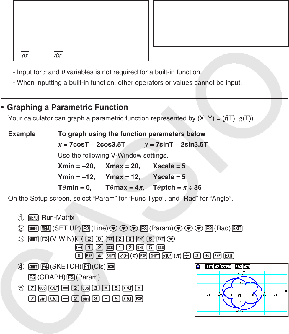
• Graphing a Parametric Function
Your calculator can graph a parametric function represented by (X, Y) = (f(T), g(T)).
Example To graph using the function parameters below
x = 7cosT − 2cos3.5T y = 7sinT − 2sin3.5T
Use the following V-Window settings.
Xmin = −20, Xmax = 20, Xscale = 5
Ymin = −12, Ymax = 12, Yscale = 5
T
θ
min = 0, T
θ
max = 4
π
, T
θ
ptch =
π
÷ 36
On the Setup screen, select “Param” for “Func Type”, and “Rad” for “Angle”.
1 m Run-Matrix
2 !m(SET UP)2(Line)ccc3(Param)ccc2(Rad)J
3 !3(V-WIN) -cawcawfwc
-bcwbcwfw
awe!5(
π
)w!5(
π
)/dgwJ
4 !4(SKETCH)1(Cls)w
5(GRAPH)3(Param)
5 hcv-ccd.fv,
hsv-csd.fvw
dx
(
x
)
d
dx
(
x
)
d
dx
2
(
x
)
d
2
dx
2
(
x
)
d
2
∫(
x
)
dx
∫(
x
)
dx