
User Manual

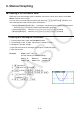
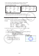
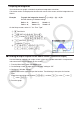
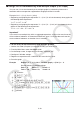
Table Of Contents
- Contents
- Getting Acquainted — Read This First!
- Chapter 1 Basic Operation
- Chapter 2 Manual Calculations
- 1. Basic Calculations
- 2. Special Functions
- 3. Specifying the Angle Unit and Display Format
- 4. Function Calculations
- 5. Numerical Calculations
- 6. Complex Number Calculations
- 7. Binary, Octal, Decimal, and Hexadecimal Calculations with Integers
- 8. Matrix Calculations
- 9. Vector Calculations
- 10. Metric Conversion Calculations
- Chapter 3 List Function
- Chapter 4 Equation Calculations
- Chapter 5 Graphing
- 1. Sample Graphs
- 2. Controlling What Appears on a Graph Screen
- 3. Drawing a Graph
- 4. Saving and Recalling Graph Screen Contents
- 5. Drawing Two Graphs on the Same Screen
- 6. Manual Graphing
- 7. Using Tables
- 8. Modifying a Graph
- 9. Dynamic Graphing
- 10. Graphing a Recursion Formula
- 11. Graphing a Conic Section
- 12. Drawing Dots, Lines, and Text on the Graph Screen (Sketch)
- 13. Function Analysis
- Chapter 6 Statistical Graphs and Calculations
- 1. Before Performing Statistical Calculations
- 2. Calculating and Graphing Single-Variable Statistical Data
- 3. Calculating and Graphing Paired-Variable Statistical Data (Curve Fitting)
- 4. Performing Statistical Calculations
- 5. Tests
- 6. Confidence Interval
- 7. Distribution
- 8. Input and Output Terms of Tests, Confidence Interval, and Distribution
- 9. Statistic Formula
- Chapter 7 Financial Calculation
- Chapter 8 Programming
- Chapter 9 Spreadsheet
- Chapter 10 eActivity
- Chapter 11 Memory Manager
- Chapter 12 System Manager
- Chapter 13 Data Communication
- Chapter 14 Geometry
- Chapter 15 Picture Plot
- Chapter 16 3D Graph Function
- Appendix
- Examination Mode
- E-CON4 Application (English)
- 1. E-CON4 Mode Overview
- 2. Sampling Screen
- 3. Auto Sensor Detection (CLAB Only)
- 4. Selecting a Sensor
- 5. Configuring the Sampling Setup
- 6. Performing Auto Sensor Calibration and Zero Adjustment
- 7. Using a Custom Probe
- 8. Using Setup Memory
- 9. Starting a Sampling Operation
- 10. Using Sample Data Memory
- 11. Using the Graph Analysis Tools to Graph Data
- 12. Graph Analysis Tool Graph Screen Operations
- 13. Calling E-CON4 Functions from an eActivity
5-21
k Saving Graph Screen Contents as an Image (g3p File)
There are two methods that can be used to save a g3p file.
• Saving to Picture Memory
This method lets you assign a number from 1 to 20 to an image when you save it. It stores
the image in the storage memory’s PICT folder as a file with a name from Pict01.g3p through
Pict20.g3p.
• Saving under an Assigned Name
This method saves the image in the folder you want in storage memory. You can assign a
file name up to eight characters long.
Important!
• A dual graph screen or any other type of graph that uses a split screen cannot be saved in
picture memory.
u To save a graph screen image to Picture Memory
1. While the graph screen is on the display, press K1(PICTURE)1(STORE)1(1-20).
2. On the Store In Picture Memory screen that appears, enter a value from 1 to 20 and then
press w.
• There are 20 picture memories numbered Pict 1 to Pict 20.
• Storing an image in a memory area that already contains an image replaces the existing
image with the new one.
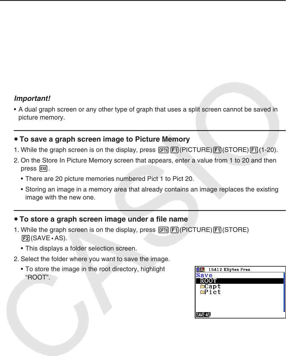
u To store a graph screen image under a file name
1. While the graph screen is on the display, press K1(PICTURE)1(STORE)
2(SAVE • AS).
• This displays a folder selection screen.
2. Select the folder where you want to save the image.
• To store the image in the root directory, highlight
“ROOT”.