
User Manual
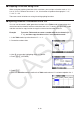
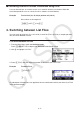
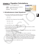
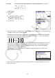
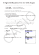
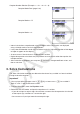
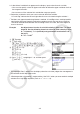
Table Of Contents
- Contents
- Getting Acquainted — Read This First!
- Chapter 1 Basic Operation
- Chapter 2 Manual Calculations
- 1. Basic Calculations
- 2. Special Functions
- 3. Specifying the Angle Unit and Display Format
- 4. Function Calculations
- 5. Numerical Calculations
- 6. Complex Number Calculations
- 7. Binary, Octal, Decimal, and Hexadecimal Calculations with Integers
- 8. Matrix Calculations
- 9. Vector Calculations
- 10. Metric Conversion Calculations
- Chapter 3 List Function
- Chapter 4 Equation Calculations
- Chapter 5 Graphing
- 1. Sample Graphs
- 2. Controlling What Appears on a Graph Screen
- 3. Drawing a Graph
- 4. Saving and Recalling Graph Screen Contents
- 5. Drawing Two Graphs on the Same Screen
- 6. Manual Graphing
- 7. Using Tables
- 8. Modifying a Graph
- 9. Dynamic Graphing
- 10. Graphing a Recursion Formula
- 11. Graphing a Conic Section
- 12. Drawing Dots, Lines, and Text on the Graph Screen (Sketch)
- 13. Function Analysis
- Chapter 6 Statistical Graphs and Calculations
- 1. Before Performing Statistical Calculations
- 2. Calculating and Graphing Single-Variable Statistical Data
- 3. Calculating and Graphing Paired-Variable Statistical Data (Curve Fitting)
- 4. Performing Statistical Calculations
- 5. Tests
- 6. Confidence Interval
- 7. Distribution
- 8. Input and Output Terms of Tests, Confidence Interval, and Distribution
- 9. Statistic Formula
- Chapter 7 Financial Calculation
- Chapter 8 Programming
- Chapter 9 Spreadsheet
- Chapter 10 eActivity
- Chapter 11 Memory Manager
- Chapter 12 System Manager
- Chapter 13 Data Communication
- Chapter 14 Geometry
- Chapter 15 Picture Plot
- Chapter 16 3D Graph Function
- Appendix
- Examination Mode
- E-CON4 Application (English)
- 1. E-CON4 Mode Overview
- 2. Sampling Screen
- 3. Auto Sensor Detection (CLAB Only)
- 4. Selecting a Sensor
- 5. Configuring the Sampling Setup
- 6. Performing Auto Sensor Calibration and Zero Adjustment
- 7. Using a Custom Probe
- 8. Using Setup Memory
- 9. Starting a Sampling Operation
- 10. Using Sample Data Memory
- 11. Using the Graph Analysis Tools to Graph Data
- 12. Graph Analysis Tool Graph Screen Operations
- 13. Calling E-CON4 Functions from an eActivity
4-3
2. High-order Equations from 2nd to 6th Degree
Your calculator can be used to solve high-order equations from 2nd to 6th degree.
• Quadratic Equation:
ax
2
+ bx + c = 0 ( a 0)
• Cubic Equation:
ax
3
+ bx
2
+ cx + d = 0 ( a 0)
• Quartic Equation:
ax
4
+ bx
3
+ cx
2
+ dx + e = 0 ( a 0)
…
1. From the Main Menu, enter the Equation mode.
2. Select the POLY (Polynomial) mode, and specify the degree of the equation.
You can specify a degree 2 to 6.
3. Sequentially input the coefficients.
• The cell that is currently selected for input is highlighted. Each time you input a coefficient,
the highlighting shifts in the sequence:
a → b → c → …
• You can also input fractions and values assigned to variables as coefficients.
• You can cancel the value you are inputting for the current coefficient by pressing J at
any time before you press w to store the coefficient value. This returns to the coefficient
to what it was before you input anything. You can then input another value if you want.
• To change the value of a coefficient that you already stored by pressing w, move the
cursor to the coefficient you want to edit. Next, input the value you want to change to.
• Pressing 3(CLEAR) clears all coefficients to zero.
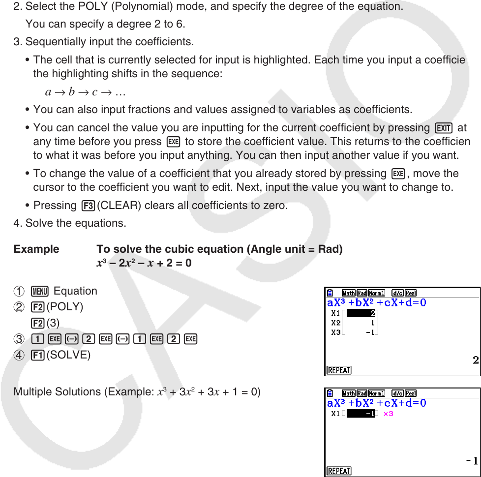
4. Solve the equations.
Example To solve the cubic equation (Angle unit = Rad)
x
3
– 2 x
2
– x + 2 = 0
1 m Equation
2 2(POLY)
2(3)
3 bw-cw-bwcw
4 1(SOLVE)
Multiple Solutions (Example: x
3
+ 3 x
2
+ 3 x + 1 = 0)