
User Manual
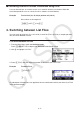
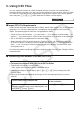
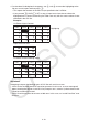
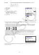
Table Of Contents
- Contents
- Getting Acquainted — Read This First!
- Chapter 1 Basic Operation
- Chapter 2 Manual Calculations
- 1. Basic Calculations
- 2. Special Functions
- 3. Specifying the Angle Unit and Display Format
- 4. Function Calculations
- 5. Numerical Calculations
- 6. Complex Number Calculations
- 7. Binary, Octal, Decimal, and Hexadecimal Calculations with Integers
- 8. Matrix Calculations
- 9. Vector Calculations
- 10. Metric Conversion Calculations
- Chapter 3 List Function
- Chapter 4 Equation Calculations
- Chapter 5 Graphing
- 1. Sample Graphs
- 2. Controlling What Appears on a Graph Screen
- 3. Drawing a Graph
- 4. Saving and Recalling Graph Screen Contents
- 5. Drawing Two Graphs on the Same Screen
- 6. Manual Graphing
- 7. Using Tables
- 8. Modifying a Graph
- 9. Dynamic Graphing
- 10. Graphing a Recursion Formula
- 11. Graphing a Conic Section
- 12. Drawing Dots, Lines, and Text on the Graph Screen (Sketch)
- 13. Function Analysis
- Chapter 6 Statistical Graphs and Calculations
- 1. Before Performing Statistical Calculations
- 2. Calculating and Graphing Single-Variable Statistical Data
- 3. Calculating and Graphing Paired-Variable Statistical Data (Curve Fitting)
- 4. Performing Statistical Calculations
- 5. Tests
- 6. Confidence Interval
- 7. Distribution
- 8. Input and Output Terms of Tests, Confidence Interval, and Distribution
- 9. Statistic Formula
- Chapter 7 Financial Calculation
- Chapter 8 Programming
- Chapter 9 Spreadsheet
- Chapter 10 eActivity
- Chapter 11 Memory Manager
- Chapter 12 System Manager
- Chapter 13 Data Communication
- Chapter 14 Geometry
- Chapter 15 Picture Plot
- Chapter 16 3D Graph Function
- Appendix
- Examination Mode
- E-CON4 Application (English)
- 1. E-CON4 Mode Overview
- 2. Sampling Screen
- 3. Auto Sensor Detection (CLAB Only)
- 4. Selecting a Sensor
- 5. Configuring the Sampling Setup
- 6. Performing Auto Sensor Calibration and Zero Adjustment
- 7. Using a Custom Probe
- 8. Using Setup Memory
- 9. Starting a Sampling Operation
- 10. Using Sample Data Memory
- 11. Using the Graph Analysis Tools to Graph Data
- 12. Graph Analysis Tool Graph Screen Operations
- 13. Calling E-CON4 Functions from an eActivity
4-2
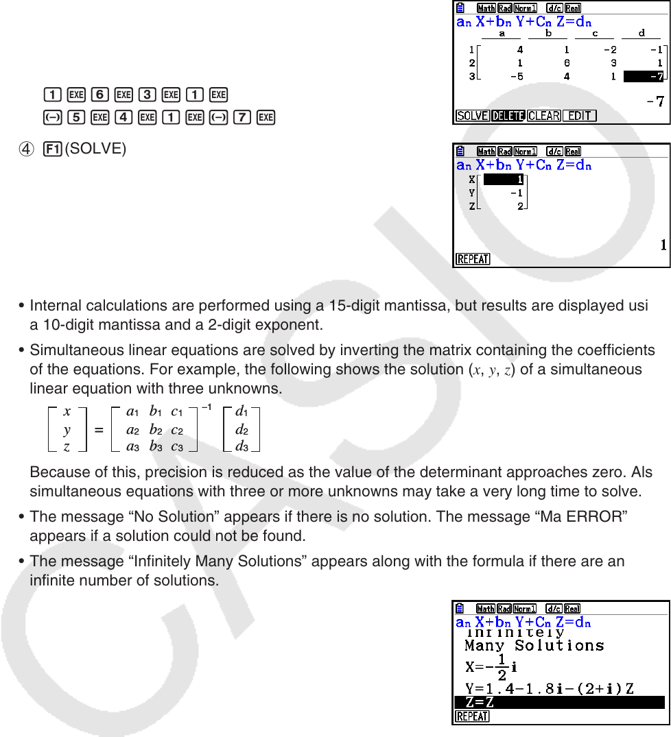
Example To solve the following simultaneous linear equations for
x , y , and z
4 x + y – 2 z = – 1
x + 6 y + 3 z = 1
– 5
x + 4 y + z = – 7
1 m Equation
2 1(SIMUL)
2(3)
3 ewbw-cw-bw
bwgwdwbw
-fwewbw-hw
4 1(SOLVE)
• Internal calculations are performed using a 15-digit mantissa, but results are displayed using
a 10-digit mantissa and a 2-digit exponent.
• Simultaneous linear equations are solved by inverting the matrix containing the coefficients
of the equations. For example, the following shows the solution ( x
, y
, z
) of a simultaneous
linear equation with three unknowns.
Because of this, precision is reduced as the value of the determinant approaches zero. Also,
simultaneous equations with three or more unknowns may take a very long time to solve.
• The message “No Solution” appears if there is no solution. The message “Ma ERROR”
appears if a solution could not be found.
• The message “Infinitely Many Solutions” appears along with the formula if there are an
infinite number of solutions.
• After calculation is complete, you can press 1(REPEAT), change coefficient values, and
then re-calculate.
–1
=
x
y
z
a
1
b
1
c
1
a
2
b
2
c
2
a
3
b
3
c
3
d
1
d
2
d
3
–1
=
x
y
z
a
1
b
1
c
1
a
2
b
2
c
2
a
3
b
3
c
3
d
1
d
2
d
3