For ClassPad 300 E Spreadsheet Application Version 2.0 User’s Guide RJA510188-4 http://classpad.
Using the Spreadsheet Application The Spreadsheet application provides you with powerful, take-along-anywhere spreadsheet capabilities on your ClassPad.
Contents 1 Contents 1 Spreadsheet Application Overview .................................................................... 1-1 Starting Up the Spreadsheet Application ....................................................................... 1-1 Spreadsheet Window ..................................................................................................... 1-1 2 Spreadsheet Application Menus and Buttons ................................................... 2-1 3 Basic Spreadsheet Window Operations ...
1-1 Spreadsheet Application Overview 1 Spreadsheet Application Overview This section describes the configuration of the Spreadsheet application window, and provides basic information about its menus and commands. Starting Up the Spreadsheet Application Use the following procedure to start up the Spreadsheet application. u ClassPad Operation (1) On the application menu, tap R. • This starts the Spreadsheet application and displays its window.
2-1 Spreadsheet Application Menus and Buttons 2 Spreadsheet Application Menus and Buttons This section explains the operations you can perform using the menus and buttons of the Spreadsheet application window. • For information about the O menu, see “Using the O Menu” on page 1-5-4 of your ClassPad 300 User’s Guide.
2-2 Spreadsheet Application Menus and Buttons k Graph Menu You can use the [Graph] menu to graph the data contained in selected cells. See “8 Graphing” for more information. k Action Menu The [Action] menu contains a selection of functions that you can use when configuring a spreadsheet. See “6 Using the Action Menu” for more information. k Spreadsheet Toolbar Buttons Not all of the Spreadsheet buttons can fit on a single toolbar, tap the u/t button on the far right to toggle between the two toolbars.
3-1 Basic Spreadsheet Window Operations 3 Basic Spreadsheet Window Operations This section contains information about how to control the appearance of the Spreadsheet window, and how to perform other basic operations. About the Cell Cursor The cell cursor causes the current selected cell or group of cells to become highlighted. The location of the current selection is indicated in the status bar, and the value or formula located in the selected cell is shown in the edit box.
3-2 Basic Spreadsheet Window Operations (2) On the dialog box that appears, tap the [Cursor Movement] down arrow button, and then select the setting you want. To have the cell cursor behave this way when you register input: Select this setting: Remain at the current cell Off Move to the next row below the current cell Down Move to the next column to the right of the current cell Right (3) After the setting is the way you want, tap [OK].
3-3 Basic Spreadsheet Window Operations k Jumping to a Cell You can use the following procedure to jump to a specific cell on the Spreadsheet screen by specifying the cell’s column and row. u ClassPad Operation (1) On the [Edit] menu, select [Goto Cell]. (2) On the dialog box that appears, type in a letter to specify the column of the cell to which you want to jump, and a value for its row number. (3) After the column and row are the way you want, tap [OK] to jump to the cell.
3-4 Basic Spreadsheet Window Operations Hiding or Displaying the Scrollbars Use the following procedure to turn display of Spreadsheet scrollbars on and off. By turning off the scrollbars, you make it possible to view more information in the spreadsheet. u ClassPad Operation (1) On the [Edit] menu, tap [Options]. (2) On the dialog box that appears, tap the [Scrollbars] down arrow button, and then select the setting you want.
3-5 Basic Spreadsheet Window Operations Selecting Cells Before performing any operation on a cell, you must first select it. You can select a single cell, a range of cells, all the cells in a row or column, or all of the cells in the spreadsheet. Tap here to select the entire spreadsheet. Tap a column heading to select the column. Tap a cell to select it. Tap a row heading to select the row. • To select a range of cells, drag the stylus across them.
3-6 Basic Spreadsheet Window Operations Using the Cell Viewer Window The Cell Viewer window lets you view both the formula contained in a cell, as well as the current value produced by the formula. While the Cell Viewer window is displayed, you can select or clear its check boxes to toggle display of the value and/or formula on or off. You can also select a value or formula and then drag it to another cell. u To view or hide the Cell Viewer window On the Spreadsheet toolbar, tap A.
4-1 Editing Cell Contents 4 Editing Cell Contents This section explains how to enter the edit mode for data input and editing, and how to input various types of data and expressions into cells. Edit Mode Screen The Spreadsheet application automatically enters the edit mode whenever you tap a cell to select it and input something from the keypad. Entering the edit mode (see page 4-2) displays the editing cursor in the edit box and the data input toolbar.
4-2 Editing Cell Contents • You can tap the data input toolbar buttons to input letters and symbols into the edit box. Entering the Edit Mode There are two ways you can enter the edit mode: • Tapping a cell and then tapping inside the edit box • Tapping a cell and inputting something on the keypad The following explains the difference between these two techniques. k Tapping a cell and then tapping the edit box • This enters the “standard” edit mode.
4-3 Editing Cell Contents k Tapping a cell and then inputting something from the keypad • This enters the “quick” edit mode, indicated by a dashed blinking cursor. Anything you input with the keypad will be displayed in the edit box. • If the cell you selected already contains something, anything you input with the quick edit mode replaces the existing content with the new input.
4-4 Editing Cell Contents Inputting a Formula A formula is an expression that the Spreadsheet application calculates and evaluates when you input it, when data related to the formula is changed, etc. A formula always starts with an equal sign (=), and can contain any one of the following.
4-5 Editing Cell Contents (3) Press k to display the soft keyboard. (4) Tap the 0 tab and then tap r, o, w, or on the [Action] menu, tap [row]. (5) Press (, tap cell A1, and then press ). (6) Press E. (7) Tap cell B1 and then press =. (8) On the soft keyboard, tap the 9 tab, tap -, and then tap -. (9) Tap cell A1, press ,, x, ,, 1, and then press ). (10) Press E. (11) Press k to hide the soft keyboard. (12) Select (highlight) cells A1 and B1. (13) On the [Edit] menu, tap [Copy].
4-6 Editing Cell Contents Inputting a Cell Reference A cell reference is a symbol that references the value of one cell for use by another cell. If you input “=A1 + B1” into cell C2, for example, the Spreadsheet will add the current value of cell A1 to the current value of cell B1, and display the result in cell C2. There are two types of cell references: relative and absolute. It is very important that you understand the difference between relative and absolute cell references.
4-7 Editing Cell Contents u To input a cell reference (1) Select the cell where you want to insert the cell reference. (2) Tap inside the edit box. (3) If you are inputting new data, input an equal sign (=) first. If you are editing existing data, make sure that its first character is an equal sign (=). • Inputting a cell name like “A3” without an equal sign (=) at the beginning will cause “A” and “3” to be input as text, without referencing the data in cell A3.
4-8 Editing Cell Contents Inputting a Constant A constant is data whose value is defined when it is input. When you input something into a cell for which text is specified as the data type without an equal sign (=) at the beginning, a numeric value is treated as a constant and non-numeric values are treated as text.
4-9 Editing Cell Contents (2) Use the dialog box that appears to configure the Fill Sequence operation as described below. Parameter Description Expr. Input the expression whose results you want to input. Var. Specify the name of the variable whose value will change with each step. Low Specify the smallest value to be assigned to the variable. High Specify the greatest value to be assigned to the variable. Step Specify the value that should be added to the variable value with each step.
4-10 Editing Cell Contents (3) After everything is the way you want, tap [OK]. • This performs all the required calculations according to your settings, and inserts the results into the spreadsheet. • The following shows the results for our example. Cut and Copy You can use the [Cut] and [Copy] commands on the Spreadsheet application [Edit] menu to cut and copy the contents of the cells currently selected (highlighted) with the cell cursor. You can also cut and copy text from the edit box.
4-11 Editing Cell Contents Paste The [Edit] menu’s [Paste] command lets you paste the data that is currently on the clipboard at the current cell cursor or editing cursor location. Important! • Pasting cell data will cause all relative cell references contained in the pasted data to be changed in accordance with the paste location. See “Inputting a Cell Reference” on page 4-6 for more information.
4-12 Editing Cell Contents • The following shows how cell data is converted to a matrix format when pasted into the edit box. Select the cell where you want to insert the text (A6 in this example), and then tap inside the edit box. Tap [Edit], and then [Paste]. To view the matrix as text, tap the cell (A6) and then A. To view the matrix as 2D, tap u to change data types.
4-13 Editing Cell Contents Specifying Text or Calculation as the Data Type for a Particular Cell A simple toolbar button operation lets you specify that the data contained in the currently selected cell or cells should be treated as either text or calculation data. The following shows how the specified data type affects how a calculation expression is handled when it is input into a cell.
4-14 Editing Cell Contents Using Drag and Drop to Copy Cell Data within a Spreadsheet You can also copy data from one cell to another within a spreadsheet using drag and drop. If the destination cell already contains data, it is replaced with the newly dropped data. • When performing this operation, you can drag and drop between cells, or from one location to another within the edit box only. You cannot drag and drop between cells and the edit box.
4-15 Editing Cell Contents k Dragging and Dropping Multiple Cells • When dragging multiple cells, only the cell where the stylus is located has a selection boundary around it. Selection boundary (cursor held against C2) • When you release the stylus from the screen, the top left cell of the group (originally A1 in the above example) will be located where you drop the selection boundary.
4-16 Editing Cell Contents u To drag and drop within the edit box (1) Select the cell whose contents you want to edit. (2) Tap the edit box to enter the edit mode. (3) Tap the edit box again to display the editing cursor (a solid blinking cursor). (4) Drag the stylus across the characters you want to move, so they are highlighted. (5) Holding the stylus against the selected characters, drag to the desired location. (6) Lift the stylus to drop the characters in place.
4-17 Editing Cell Contents u To use drag and drop to obtain the data points of a graph Example: To obtain the data points of the bar graph shown below (1) Input data and draw a bar graph. • See “Other Graph Window Operations” on page 8-13 for more information on graphing. (2) Tap the Graph window to make it active. (3) Tap the top of any bar within the Graph window, and then drag to the cell you want in the Spreadsheet window.
5-1 Using the Spreadsheet Application with the eActivity Application 5 Using the Spreadsheet Application with the eActivity Application You can display the Spreadsheet application from within the eActivity application. This makes it possible to drag data between the Spreadsheet and eActivity windows as desired. Drag and Drop After you open Spreadsheet within eActivity, you can drag and drop information between the two application windows.
5-2 Using the Spreadsheet Application with the eActivity Application (4) Select the cell you want and drag it to the first available line in the eActivity window. • This inserts the contents of the cell in the eActivity window. (5) You can now experiment with the data in the eActivity window. Example 2: To drag a calculation expression from the Spreadsheet edit box to the eActivity window u ClassPad Operation (1) Tap m to display the application menu, and then tap A to start the eActivity application.
5-3 Using the Spreadsheet Application with the eActivity Application (5) Drag the contents of the edit box to the first available line in the eActivity window. • This inserts the contents of the edit box in the eActivity window as a text string. (6) You can now experiment with the data in the eActivity window. • The basic operations for the following example are the same for the other examples described above.
5-4 Using the Spreadsheet Application with the eActivity Application Example 4: Dragging data from eActivity to the Spreadsheet window 20040801
6-1 Using the Action Menu 6 Using the Action Menu Most of the functions that are available from the [Action] menu are similar to those on the [List-Calculation] sub-menu of the standard [Action] menu. Spreadsheet [Action] Menu Basics The following example demonstrates the basic procedure for using functions within the [Action] menu.
6-2 Using the Action Menu uClassPad Operation (1) With the stylus, tap the cell where you want the result to appear. • In this example, we would tap cell A1. (2) On the [Action] menu, tap [sum]. • This inputs an equal sign and the [sum] function into the edit box. (3) Use the stylus to drag across the range of data cells from A7 to C12 to select them. • “A7:C12” appears to the right of the open parenthesis of the [sum] function.
6-3 Using the Action Menu (4) Tap the s button to the right of the edit box. • This automatically closes the parentheses, calculates the sum of the values in the selected range, and displays the result in cell A1. • You could skip this step and input the closing parentheses by pressing the ) key on the keypad, if you want. (5) Tap the edit box to activate it again, and then tap to the right of the last parenthesis. (6) Press the + key and then input 100. (7) Tap the s button to the right of the edit box.
6-4 Using the Action Menu Action Menu Functions This section describes how to use each function in the [Action] menu. Please note that start cell:end cell is equivalent to entering a list. u min Function: Returns the lowest value contained in the range of specified cells.
6-5 Using the Action Menu u mean Function: Returns the mean of the values contained in the range of specified cells. Syntax: mean(start cell:end cell[,start cell:end cell]) Example: To determine the mean of the values in the block whose upper left corner is located at A7 and whose lower right corner is located at C12, and input the result in cell A1: u median Function: Returns the median of the values contained in the range of specified cells.
6-6 Using the Action Menu u mode Function: Returns the mode of the values contained in the range of specified cells. Syntax: mode(start cell:end cell[,start cell:end cell]) Example: To determine the mode of the values in the block whose upper left corner is located at A7 and whose lower right corner is located at C12, and input the result in cell A1: u sum Function: Returns the sum of the values contained in the range of specified cells.
6-7 Using the Action Menu u prod Function: Returns the product of the values contained in the range of specified cells. Syntax: prod(start cell:end cell[,start cell:end cell]) Example: To determine the product of the values in cells A7 and A8, and input the result in cell A1: u cuml Function: Returns the cumulative sums of the values contained in the range of specified cells.
6-8 Using the Action Menu u Alist Function: Returns the differences between values in each of the adjacent cells in the range of specified cells. Syntax: Alist(start cell:end cell) Example: To determine the differences of the values in cells B1 through B3, and input the result in cell A1: u stdDev Function: Returns the sample standard deviation of the values contained in the range of specified cells.
6-9 Using the Action Menu u variance Function: Returns the sample variance of the values contained in the range of specified cells. Syntax: variance(start cell:end cell) Example: To determine the sample variance of the values in the block whose upper left corner is located at A7 and whose lower right corner is located at C12, and input the result in cell A1: u Q1 Function: Returns the first quartile of the values contained in the range of specified cells.
6-10 Using the Action Menu u Q3 Function: Returns the third quartile of the values contained in the range of specified cells. Syntax: Q3(start cell:end cell[,start cell:end cell]) Example: To determine the third quartile of the values in the block whose upper left corner is located at A7 and whose lower right corner is located at C12, and input the result in cell A1: u percent Function: Returns the percentage of each value in the range of specified cells, the sum of which is 100%.
6-11 Using the Action Menu u polyEval Function: Returns a polynomial arranged in descending order. The coefficients correspond sequentially to each value in the range of specified cells. Syntax: polyEval(start cell:end cell[,start cell:end cell] / [, variable]) Example: To create a second degree polynomial with coefficients that correspond to the values in cells B1 through B3, and input the result in cell A1: • “x” is the default variable when you do not specify one above.
6-12 Using the Action Menu u sequence Function: Returns the lowest-degree polynomial that generates the sequence expressed by the values in a list or range of specified cells. If we evaluate the polynomial at 2, for example, the result will be the second value in our list.
6-13 Using the Action Menu u sumSeq Function: Determines the lowest-degree polynomial that generates the sum of the first n terms of your sequence. If we evaluate the resulting polynomial at 1, for example, the result will be the first value in your list. If we evaluate the resulting polynomial at 2, the result will be the sum of the first two values in your list. When two columns of values or two lists are specified, the resulting polynomial returns a sum based on a sequence.
6-14 Using the Action Menu u row Function: Returns the row number of a specified cell. Syntax: row(cell) Example: To determine the row number of cell A7 and input the result in cell A1: u col Function: Returns the column number of a specified cell.
6-15 Using the Action Menu u count Function: Returns a count of the number of cells in the specified range.
7-1 Formatting Cells and Data 7 Formatting Cells and Data This section explains how to control the format of the spreadsheet and the data contained in the cells. Standard (Fractional) and Decimal (Approximate) Modes You can use the following procedure to control whether a specific cell, row, or column, or the entire spreadsheet should use the standard mode (fractional format) or decimal mode (approximate value). u ClassPad Operation (1) Select the cell(s) whose format you want to specify.
7-2 Formatting Cells and Data Text Alignment With the following procedure, you can specify justified, align left, center, or align right for a specific cell, row, or column, or the entire spreadsheet. u ClassPad Operation (1) Select the cell(s) whose alignment setting you want to specify. • See “Selecting Cells” on page 3-5 for information about selecting cells. (2) On the toolbar, tap the down arrow button next to the [ button.
7-3 Formatting Cells and Data Changing the Width of a Column There are three different methods you can use to control the width of a column: dragging with the stylus, using the [Column Width] command, or using the [AutoFit Selection] command. u To change the width of a column using the stylus Use the stylus to drag the edge of a column header left or right until it is the desired width.
7-4 Formatting Cells and Data (3) On the dialog box that appears, enter a value in the [Width] box to specify the desired width of the column in pixels. • You can also use the [Range] box to specify a different column from the one you selected in step (1) above, or a range of columns. Entering B1:D1 in the [Range] box, for example, will change columns B, C, and D to the width you specify. (4) After everything is the way you want, tap [OK] to change the column width.
7-5 Formatting Cells and Data (3) On the [Edit] menu, tap [AutoFit Selection]. • This causes the column width to be adjusted automatically so the entire value can be displayed. • Note that [AutoFit Selection] also will reduce the width of a column, if applicable. The following shows what happens when [AutoFit Selection] is executed while a cell that contains a single digit is selected.
8-1 Graphing 8 Graphing The Spreadsheet application lets you draw a variety of different graphs for analyzing data. You can combine line and column graphs, and the interactive editing feature lets you change a graph by dragging its points on the display. Graph Menu After selecting data on the spreadsheet, use the [Graph] menu to select the type of graph you want to draw. You can also use the [Graph] menu to specify whether to graph data by column or row.
8-2 Graphing u [Graph] - [Line] - [Clustered] ( D ) u [Graph] - [Line] - [Stacked] ( F ) 20040801
8-3 Graphing u [Graph] - [Line] - [100% Stacked] ( G ) u [Graph] - [Column] - [Clustered] ( H ) 20040801
8-4 Graphing u [Graph] - [Column] - [Stacked] ( J ) u [Graph] - [Column] - [100% Stacked] ( K ) 20040801
8-5 Graphing u [Graph] - [Bar] - [Clustered] ( L ) u [Graph] - [Bar] - [Stacked] ( : ) 20040801
8-6 Graphing u [Graph] - [Bar] - [100% Stacked] ( " ) u [Graph] - [Pie] ( Z ) • When you select a pie chart, only the first series (row or column) of the selected data is used. • Tapping any of the sections of a pie graph causes three values to appear at the bottom of the screen: the cell location, a data value for the section, and a percent value that indicates the portion of the total data that the data value represents.
8-7 Graphing u [Graph] - [Scatter] ( X ) • In the case of a scatter graph, the first series (column or row) of selected values is used as the x-values for all plots. The other selected values are used as the y-value for each of the plots. This means if you select four columns of data (like Columns A, B, C, and D), for example, there will be three different plot point types: (A, B), (A, C), and (A, D). • Scatter graphs initially have plotted points only.
8-8 Graphing u [Graph] - [Column Series] Selecting this option treats each column as a separate set of data. The value in each row is plotted as a vertical axis value. The following shows a typical clustered column graph while [Column Series] is selected, and the data that produced it. Graph Window Menus and Toolbar The following describes the special menus and toolbar that appears whenever the Spreadsheet application Graph window is on the display.
8-9 Graphing k View Menu Many of the [View] menu commands can also be executed by tapping Spreadsheet application Graph window toolbar buttons.
8-10 Graphing Tap this toolbar button: To do this: Or select this [Series] menu item: Display a linear regression curve d Trend - Linear Display a quadratic regression curve f Trend - Polynomial Quadratic Display a cubic regression curve g Trend - Polynomial Cubic Display a quartic regression curve h Trend - Polynomial Quartic Display a quintic regression curve j Trend - Polynomial Quintic Display an exponential AeBx regression curve k Trend - Exponential Display a logarithmic Aln(x) +
8-11 Graphing Basic Graphing Steps The following are the basic steps for graphing spreadsheet data. u ClassPad Operation (1) Input the data you want to graph into the spreadsheet. (2) Use the [Graph] menu to specify whether you want to graph the data by row or by column. To do this: Select this [Graph] menu option: Graph the data by row Row Series Graph the data by column Column Series • See “Graph Menu” on page 8-1 for more information. (3) Select the cells that contain the data you want to graph.
8-12 Graphing (4) On the [Graph] menu, select the type of graph you want to draw. Or you can tap the applicable icon on the toolbar. • This draws the selected graph. See “Graph Menu” on page 8-1 for examples of the different types of graphs that are available. • You can change to another type of graph at any time by selecting the graph type you want on the [Type] menu. Or you can tap the applicable icon on the toolbar.
8-13 Graphing Other Graph Window Operations This section provides more details about the types of operations you can perform while the Graph window is on the display. u To show or hide lines and markers (1) While a line graph or a scatter graph is on the Graph window, tap the [View] menu. Lines and markers both turned on (2) Tap the [Markers] or [Lines] item to toggle it between show (checkbox selected) and hide (checkbox cleared).
8-14 Graphing u To change a line in a clustered line graph to a column graph (1) Draw the clustered line graph. (2) With the stylus, tap any data point on the line you wish to change to a column graph. (3) On the [Series] menu, tap [Column]. • You could also tap the down arrow button next to the third tool button from the left, and then tap '. • You can change more than one line to a column graph, if you want.
8-15 Graphing u To change a column in a clustered column graph to a line (1) Draw the clustered column graph. (2) With the stylus, tap any one of the columns you wish to change to a line graph. (3) On the [Series] menu, tap [Line]. • You could also tap the down arrow button next to the third tool button from the left, and then tap z. • You can change more than one column to a line graph, if you want.
8-16 Graphing u To display a regression curve (1) Draw a clustered line graph or clustered column graph. • A regression curve can be drawn for a line, column, or scatter graph only. • The above shows a stacked line graph. (2) With the stylus, tap any point of the data for which you want to draw the regression curve. (3) Use the [Series] menu to select the type of regression curve you want.
8-17 Graphing • This causes the applicable regression curve to appear in the Graph window. • Tapping the regression curve selects it and displays its equation in the status bar. • You can drag and drop the regression curve to a cell or the edit box in the Spreadsheet window. • To delete all displayed regression curves, select [Clear All] on the [Edit] menu. • Note that regression curves are also deleted automatically if you change to another graph style.
8-18 Graphing u To find out the percentage of data for each pie graph section (1) While the display is split between the pie graph and the Spreadsheet windows, tap the pie graph to select it. (2) On the [Edit] menu, tap [Copy]. (3) Tap the Spreadsheet window to make it active. (4) Tap the cell where you want to paste the data. • The cell you tap will be the upper left cell of the group of cells that will be pasted. (5) On the [Edit] menu, tap [Paste]. • This pastes two columns of values.
8-19 Graphing u To change the appearance of the axes While a graph is on the Graph window, select [Toggle Axes] on the [View] menu or tap the q toolbar button to cycle through axes settings in the following sequence: axes on → axes and values on → axes and values off →. u To change the appearance of a graph by dragging a point While a graph is on the Graph window, use the stylus to drag any one of its data points to change the configuration of the graph.
8-20 Graphing • If a regression curve is displayed for the data whose graph is being changed by dragging, the regression curve also changes automatically in accordance with the drag changes. • When you edit data in the spreadsheet and press E, your graph will update automatically. Important! • You can drag a point only if it corresponds to a fixed value on the spreadsheet. You cannot drag a point if it corresponds to a formula.
CASIO COMPUTER CO., LTD.