E ClassPad II Examples CASIO Education website URL http://edu.casio.com Access the URL below and register as a user. http://edu.casio.
Contents Chapter 2: Main Application ................................................................................................. 3 Chapter 3: Graph & Table Application ............................................................................... 12 Chapter 4: Conics Application ........................................................................................... 18 Chapter 5: Differential Equation Graph Application.........................................................
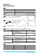
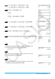
Chapter 2: Main Application 0201 Calculation Key Operation 56 × (–12) ÷ (–2.5) = 268.8 56*(z12)/(z2.5)E 2 + 3 × (4 + 5) = 29 2+3*(4+5)E = 6/(4*5)E or N*6c4*5E * The soft keyboard [Math1] key set 0202 0203 2.54 × 103 = 2540 2.54e3E 1600 × 10–4 = 0.16 bgaaE-ew 123 + 456 = 579 123+456E 789 – 579 = 210 789-DE 210 ÷ 7 = 30 /7E 0204 x:=123E 0205 Tapping u while the ClassPad is configured for Standard mode (Normal 1) display Expression 100 ÷ 6 = 16.6666666...
0208 (Assistant mode and Algebra mode calculation results) Expression Assistant Mode x + 2x + 3x + 6 expand ((x+1)2) x + 1 (When 1 is assigned to x) 0209 Algebra Mode x + 2·x + 3·x + 6 x2 + 2 · x · 1 + 12 x+1 2 2 1. Tap location 1. x2 + 5 · x + 6 x2 + 2 · x + 1 2 2.
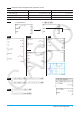
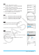
0216 5Wlista[2]E Tip: You can also perform the above operations on the “ans” variable when it contains LIST data. Example: {1, 2, 3} E {1, 2, 3} D[2]E 2 0217 list3*{6,0,4}E 0218 {10,20,30}W{x,y,Z} E 0219 [[1,2][3,4]]Wmat1E or [d[d1,2e[d3,4eeW mat1E 0220 mat1[2,1]E ↑ Row 0221 ↑ Column 5Wmat1[1,2]E Tip: You can also perform the above operations on the “ans” variable when it contains MATRIX data. 0222 1. 6 (Creates a 1-row × 2-column matrix.) 1e2 2. 6 (Adds one column to the matrix.) 3 3.
0223 [[1,1][2,1]]+ [[2,3][2,1]]E 0224 81e1cd2e1 e* 82e3cd2e1E 0225 [[1,2][3,4]]*5E 0226 [[1,2][3,4]]{3E 0227 81e2cd3e4em3E 0228 710c20730eW7xcy7ZE 0229 1. Tap the down arrow button next to the < button, and then tap 1. 2. 10111+11010E 0230 1. Tap the down arrow button next to the < button, and then tap 2. 2. (11+7){2E 0231 1. Tap the down arrow button next to the < button, and then tap 4. 2.
0232 10102 and 11002 = 10002 (Number base: Binary) 1010pandp1100E 10112 or 110102 = 110112 (Number base: Binary) 1011porp11010E 10102 xor 11002 = 1102 (Number base: Binary) 1010pxorp1100E not (FFFF16) = FFFF000016 (Number base: Hexadecimal) not(ffff)E 0233 baseConvert( 579,15,12)E baseConvert( 100,13,10)E baseConvert( 123,16,3)E 0234 1. x{3-3x{2+3x-1 2. Drag the stylus across the expression to select it. 3. Tap [Interactive], [Transformation], [factor], and then [factor]. 0235 1. x{2+2x 2.
0236 1. Input the calculation below and execute it. diff(sin(x),x) × cos(x) + sin(x) × diff(cos(x),x) 2. Drag the stylus across “diff(sin(x),x)” to select it. 3. Tap [Interactive], [Assistant] and then [apply]. • This executes the part of the calculation you selected in step 2. The part of the calculation that is not selected (× cos(x) + sin(x) × diff(cos(x),x)) is output to the display as-is. 0237 1. Tap ! to display the Graph Editor window in the lower window. 2.
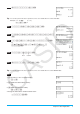
0239 1. On the work area window, tap ( to display the Stat Editor window in the lower window. 2. In the Stat Editor window, input {1, 2, 3} into “list1” and {4, 5, 6} into “list2”. 3. Make the work area window active, press k, and then perform the following calculation: list1 + list2 ⇒ list3. 4. Press k to hide the keyboard. • Here you can see that list3 contains the result of list1 + list2. 0240 1. Tap the Main application work area window to make it active. 2.
0241 1. Input the expression x^2/5^2 + y^2/2^2 = 1 in the work area. 2. Tap 3 to display the Geometry window in the lower window. 3. Drag the stylus across the expression in the work area to select it, and then drag the selected expression to the Geometry window. • An ellipse appears in the Geometry window. 0242 Point Circle A point and its image 0243 1. Start up Verify. 2. Input 50 and press E. 3. Following the equal sign (=), input 25 × 3 and press E. 4.
0244 1. Tap O and then tap [OK] to clear the window. 2. Tap the down arrow on the toolbar and select T. 3. Input x^2 + 1 and press E. 4. Input (x + i)(x – i) and press E. 0245 1. Start up Probability, and then select “2 Dice +”. 2. Enter 50 into the “Number of trials” box. 3. Tap [OK] to display the result in the Probability window. 0246 1. Tap P to display the Probability dialog box, and then select “Container”. 2. Configure the following settings on the dialog box.
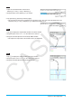
Chapter 3: Graph & Table Application 0301 1. On the a menu, tap [Draw Shade]. 2. On the dialog box that appears, input the following: Lower Func: x2 – 1, Upper Func: –x2 + 1. Leave x min and x max blank. 3. Tap [OK]. 0302 1. Tap 8 to display the Table Input dialog box, and then configure it with the settings below. Start: –4.9, End: 7.1, Step: 2 2. On the Graph Editor window, input and store y = 3log(x + 5) into line y1, and then tap #. • This generates a number table and displays it. 3.
4. Tap the Graph window to make it active. Next, tap [Analysis] and then [Trace]. • This causes a pointer to appear on the graph. 5. Use the cursor key to move the pointer along the graph until it reaches a point whose coordinates you want to input into the table. 6. Press E to input the coordinates at the current cursor position at the end of the table. 7. Repeat steps 5 and 6 to input the rest of the coordinates you want. 0304 1.
0307 1. On the Graph Editor window, input and store y = x + 1 into line y1 and y = x2 into y2, and then tap $ to graph them. 2. Tap [Analysis], [G-Solve], and then [Intersection]. • This causes “Intersection” to appear on the Graph window, with a pointer located at the point of intersection. The x- and y-coordinates at the current pointer location are also shown on the Graph window. 3.
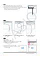
0309 1. On the Graph Editor window, input and store y = x (x + 2)(x – 2) into line y1, and then tap $ to graph it. 2. Tap [Analysis], [G-Solve], [Integral], and then [∫ dx]. • This displays “Lower” on the Graph window. 3. Press 1. • This displays a dialog box for inputting an interval for the x-values, with 1 specified for the lower limit of the x-axis (Lower). 4. Tap the [Upper] input box and then input 2 for the upper limit of the x-axis. 5. Tap [OK]. 0310 1.
0312 1. If the graph controller is not displayed on the Graph window, perform the operation below. (1) Tap O and then [Graph Format] to display the Graph Format dialog box. (2) Select the “G-Controller” check box. (3) Tap [Set]. 2. On the Graph Editor window, input 2x2 + 3x – 1 in line y1, and 2x + 1 in line y2. 3. Tap $ to graph the function. 4. Tap [Analysis] and then [Modify]. • This displays a dialog box for inputting the step. 5.
7. Configure the following settings on the Dynamic Graph dialog box. Setting Description Modify: Manual Specifies whether graph modify should be performed manually using the cursor keys (or graph controller arrows) or automatically. Dynamic ]': a Specifies a variable whose value is changed when you press the left or right cursor key, or tap the left or right graph controller arrow.
Chapter 4: Conics Application 0401 1. On the Conics Editor window, tap q to display the Select Conics Form dialog box. 2. Select “x = A(y – K)2 + H” and then tap [OK]. • This inputs “x = A(y – K)2 + H” in the Conics Editor window. 3. Change the coefficients of the equation as follows: A = 2, K = 1, H = –2. 4. Tap ^ to graph the equation. 0402 1. On the Conics Editor window, input the equation ( − 1)2 2 . + ( − 2)2 = 2 2 4 2.
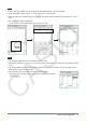
Chapter 5: Differential Equation Graph Application 0501 1. On the Differential Equation Editor window, tap [Type] - [1st (Slope Field)] or A. 2. Y{c-Xw 3. Tap O to draw the slope field. 4. Tap 6, and configure the View Window settings as shown below. 5. Tap [OK]. This updates the slope field in accordance with the new View Window settings. 0502 1. Activate the Differential Equation Editor window and then tap the [IC] tab. • This displays the initial condition editor. 2.
0503 1. On the Differential Equation Editor window, tap [Type] - [2nd (Phase Plane)] or B. 3. Tap O to draw the phase plane. 2. Xw-Yw 0504 1. Activate the Differential Equation Editor window and then tap the [IC] tab. • This displays the initial condition editor. 2. Input (xi, yi) = (1, 1) on the initial condition editor. 3. Tap O. • This graphs the solution curve and overlays it on the phase plane of x’ = x, y’ = −y. 0505 1. On the Differential Equation Editor window, tap [Type] - [Nth (No Field)] or 9.
0506 1. On the Differential Equation Editor window, tap the [Graphs] tab. 2. Tap [Type] - [ f (x)] or d, and then input y = x2 and y = −x2. 3. Tap O. • This will overlay the graphs of y = x2 and y = −x2 on the differential equation graph. 0507 1. On the Differential Equation Editor window, tap the [Graphs] tab. 2. Confirm that “Rad” is displayed as the angle unit setting on the left side of the status bar. If it isn’t, tap the angle setting until “Rad” is displayed. 3.
0508 1. Start up the eActivity application and input the following expression and matrix. y’ = exp(x) + x2 [0,1] 2. From the eActivity application menu, tap [Insert], [Strip(2)], and then [DiffEqGraph]. • This inserts a Differential Equation Graph data strip, and displays the Differential Equation Graph window in the lower half of the screen. 3. Drag the stylus across “y’ = exp(x) + x2” on the eActivity application window to select it. 4.
0509 1. Start up the eActivity application and input the following expression and matrix. y” + y’ = exp(x) [[0,1,0][0,2,0]] 2. From the eActivity application menu, tap [Insert], [Strip(2)], and then [DiffEqGraph]. • This inserts a Differential Equation Graph data strip, and displays the Differential Equation Graph window in the lower half of the screen. 3. Drag the stylus across “y” + y’ = exp(x)” on the eActivity application window to select it. 4.
Chapter 6: Sequence Application 0601 1. On the Sequence Editor window, tap the [Recursive] tab. 2. Tap [Type] - [an+2Type a1,a2]. 3. Input the recursion expression an+2 = an+1 + an and the initial values a1 = 1, a2 = 1. 4. Tap 8 to display the Sequence Table Input dialog box. 5. Input the n-value range as shown below, and then tap [OK]. Start: 1 End: 5 6. Tap the down arrow button next to #, and then select ` to create the table. −3 = 2 + 1 0602 1.
0604 1. On the Sequence Editor window, tap the [Recursive] tab. 2. Tap [Type] - [an+1Type a1]. 3. Input the recursion expression an+1 = 2an + 1 and the initial values a1 = 1. 4. Tap the down arrow button next to #, and then select + to create the table. 5. Tap 6, configure View Window settings as shown below, and then tap [OK]. xmin = 0 xmax = 6 xscale = 1 xdot: (Specify auto setting.) ymin = –15 ymax = 65 yscale = 5 ydot: (Specify auto setting.) 6.
Chapter 7: Statistics Application 0701 1. On the Stat Editor window, input the two lists (list1 = 0.5, 1.2, 2.4, 4.0, 5.2, list2 = −2.1, 0.3, 1.5, 2.0, 2.4). 2. Tap G to display the Set StatGraphs dialog box. 3. Configure the settings shown in the screen to the right and then tap [Set]. 4. Tap y to draw the scatter plot. 0702 1. On the Stat Editor window, tap [Calc] - [Test] . 2. Select [One-Sample Z-Test] and [Variable], and then tap [Next>>]. 3. Select the condition [⫽] and input values.
0704 1. On the Stat Editor window, tap ~ to display the Main application work area window. 2. Input the matrix 11 68 3 and assign it to variable a (see “2-5 Matrix and 9 23 5 Vector Calculations” in the User’s Guide). 3. Tap the Stat Editor window to make it active. 4. Tap [Calc] - [Test] - [χ2 Test] and then tap [Next>>]. 5. Input “a” in the Matrix dialog box, and then tap [Next>>]. • This displays the calculation results. 6. Tap $ to graph the results. 0705 1.
0707 1. On the Stat Editor window, tap ~ to display the Main application work area window. 2. Assign {113,116} to list1, {139,132} to list2, {133,131} to list3, and {126,122} to list4 (see “2-4 List Calculations” in the User’s Guide). 3. Tap the Stat Editor window to make it active. 4. Tap [Calc] - [Test] - [Two-Way ANOVA] and then tap [Next>>]. 5. Select “2 × 2” as the dimensions of the ANOVA data table, and then tap [Next>>]. 6.
0709 [Normal PD] 0710 [Normal CD] 0711 [Inverse Normal CD] 0712 [Poisson PD] 0713 [Poisson CD] 0714 [Inverse Poisson CD] Tip: Graphing the results of one of the following calculations may take a long time when the absolute value of the argument is large: Binomial PD, Binomial CD, Poisson PD, Poisson CD, Geometric PD, Geometric CD, Hypergeometric PD, or Hypergeometric CD calculations.
Chapter 8: Geometry Application 0801 1. Draw the triangle. 2. Tap G. Next, tap side AB and then side AC to select them. 3. Tap the u button to the right of the toolbar. • This displays the measurement box, which indicates the specified angle. 4. Tap [Draw], [Measurement], and then [angle]. • This shows the angle measurement on the screen. • You can also perform the operation below in place of step 4. - Select (highlight) value in the measurement box and drop it into the Geometry window.
0803 1. Tap [Draw], [Special Polygon], and then [Regular n-gon]. • This displays the n-gon dialog box. 2. Enter a value indicating the number of sides of the polygon, and then tap [OK]. 3. Place the stylus on the screen and drag diagonally in any direction. • This causes a selection boundary to appear, indicating the size of the polygon that will be drawn. The polygon is drawn when you release the stylus. 0804 1. Draw a line segment AB and plot point C, which is not on line segment AB. 2.
Chapter 9: Numeric Solver Application 0901 1. On the Numeric Solver window, input the equation: h = vt – 1/2 gt2 2. On the list of expression variables that appears, enter values for the variables: h = 14, t = 2, and g = 9.8. 3. Here, we will solve for v, so tap the option button to the left of variable v. 4. Tap 1. • The [Left–Right] value shows the difference between the left side and right side results.
Chapter 10: eActivity Application 1001 1. On the eActivity window, tap [Insert], [Strip(1)], and then [Graph]. • This inserts a Graph strip, and displays the Graph window in the lower half of the screen. 2. On the Graph window, tap ! to display the Graph Editor window. 3. Enter functions to graph, and then tap $ to graph the functions. eActivity window Graph Editor window Graph window 4. After you finish performing the operation you want, tap C to close the Graph window. 5.
Chapter 11: Financial Application The operations in the examples below can be started from any Financial application window. 1101 Compound Interest What will be the value of an ordinary annuity at the end of 10 years if $100 is deposited each month into an account that earns 7% compounded monthly? Before performing the calculation, change the “Odd Period” setting to “Compound (CI)” and the “Payment Date” to “End of period”. 1. Tap [Calc(1)] - [Compound Interest]. 2.
Page 2 (Amortization): Use the monthly payment value you obtained on Page 1 (PMT = –837.9966279) to determine the following information for payment 10 (PM1) through 15 (PM2).
1107 Depreciation Use the sum-of-the-years’-digits method ([SYD]) to calculate the first year ( j = 1) of depreciation on an $12,000 (PV) computer, with a useful life (N) of five years. Use a depreciation ratio (I%) of 25%, and assume that the computer can be depreciated for a full 12 months in the first year (YR1). Next, calculate the depreciation amount ([SYD]) for the second year ( j = 2). Calculate the depreciation amount for the first year: 1. Tap [Calc(1)] - [Depreciation]. 2.
1109 Break-Even Point Your company is producing items with a unit variable cost ([VCU]) of $50/ unit and fixed costs ([FC]) of $100,000. The items will be sold for a sales price ([PRC]) of $100/unit. What is the break-even point sales amount ([SBE]) and sales quantity ([QBE]) required for a profit ([PRF]) of $400,000? Before performing the calculation, change the “Profit Amount/Ratio” setting to “Amount (PRF)” and the “Break-Even Value” to “Quantity”. 1. Tap [Calc(2)] - [Break-Even Point]. 2.
1114 Quantity Conversion Calculate the sales quantity (Sales: [QTY]) when the sales amount ([SAL]) is $100,000 and the sales price ([PRC]) is $200 per unit. Next, calculate the total variable costs of production (Manufacturing: [VC]) when the variable cost per unit ([VCU]) is $30 and the number of units manufactured ([QTY]) is 500. 1. Tap [Calc(2)] - [Quantity Conversion]. 2. Input 100000 into the [SAL] field and 200 into the [PRC] field, and then tap [QTY]. 3.
Chapter 12: Program Application Note: The notation in the “Program” uses 䡺 to represent a space and _ for a carriage return. 1201 Program: DefaultSetup_ ClrGraph_ ViewWindow_ SetInequalityPlot䡺 Intersection_ GraphType䡺"y>"_ Define䡺y1(x)=sin(x)_ GTSelOn䡺1_ PTDot䡺1_ SheetActive䡺1_ DrawGraph_ GraphType䡺"y<"_ Define䡺y2(x)=−x/12_ GTSelOn䡺2_ PTNormal䡺2_ SheetActive䡺1_ DrawGraph 1203 Program: DefaultSetup_ ClrGraph_ ViewWindow䡺0,7.
Note: MedMed, QuadR, CubicR, QuartR, LinearR, ExpR, abExpR, or PowerR can also be specified in instead of LogR for the graph type. 1207 Program: {0.5,1.2,2.4,4,5.2}Slist1_ {–2.1,0.3,1.5,2,2.4}Slist2_ StatGraph䡺1, On, SinR, list1, list2_ DrawStat 1209 Program: {7,4,6,6,5,6,5,5,8,7,4,7,6,7,6} Slist1_ {1,1,1,1,1,2,2,2,2,2,3,3,3,3,3} Slist2_ OneWayANOVA䡺list1, list2_ DispStat 1211 Program: OneSampleZTest䡺"≠",0,3,24.
Chapter 13: Spreadsheet Application 1301 1. On the Spreadsheet window, input the data and then select input range cells A1:C5. 2. Tap [Calc] - [Test] - [Linear Reg t-Test], and then tap [Next>>]. • This will automatically insert the cell references into the fields as shown in the nearby screen shot. 3. Tap [Next>>]. 4. Tap $ to draw the linear regression graph. 1302 1. On the Spreadsheet window, input the data and then select input range cells A1:D2. 2.
1304 1. Input values into cells A1 through C3. 2. Tap cell C5. Next, on the [Calc] menu, tap [List-Statistics] and then [mean]. • This will input “=mean(” into the cell. 3. Drag from cell A1 to cell C3 to input the cell reference “A1:C3”. 4. Tap the s button next to the edit box or press the E key. 1305 1. Input values into cells A1 through B3. 2. Tap cell B5. Next, on the [Calc] menu, tap [List-Calculation] and then [sum]. 3. Drag from cell A1 to cell A3 to input the cell reference “A1:A3”. 4.
CASIO COMPUTER CO., LTD. 6-2, Hon-machi 1-chome Shibuya-ku, Tokyo 151-8543, Japan One or more of the following patents may be used in the product. U.S.Pats.