E ClassPad II fx-CP400 User’s Guide CASIO Education website URL https://edu.casio.com Download Free trial software and Support software https://edu.casio.com/dl/ Manuals are available in multi languages at https://world.casio.
Be sure to keep physical records of all important data! Low battery power or incorrect replacement of the batteries that power the ClassPad can cause the data stored in memory to be corrupted or even lost entirely. Stored data can also be affected by strong electrostatic charge or strong impact. It is up to you to keep backup copies of data to protect against its loss. Backing Up Data ClassPad data can be converted to a VCP file or XCP file and transferred to a computer for storage.
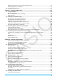
Contents About This User’s Guide .......................................................................................................................... 11 Chapter 1: Basics ................................................................................................................ 12 1-1 General Guide .........................................................................................................................12 ClassPad at a Glance........................................................
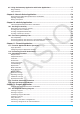
Using a List in a Calculation ..................................................................................................................... 57 Using a List to Assign Different Values to Multiple Variables ................................................................... 57 2-5 Matrix and Vector Calculations .............................................................................................58 Inputting Matrix Data ..........................................................................
Scrolling the Graph Window ................................................................................................................... 105 Zooming the Graph Window................................................................................................................... 105 Using Quick Zoom .................................................................................................................................. 106 Using Built-in Functions for Graphing................................
Determining the General Term of a Recursion Expression .................................................................... 131 Calculating the Sum of a Sequence ....................................................................................................... 131 6-2 Graphing a Recursion ..........................................................................................................131 Chapter 7: Statistics Application .......................................................................
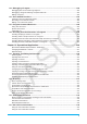
8-5 Using the Geometry Application with Other Applications ................................................177 Drag and Drop ........................................................................................................................................ 177 Copy and Paste ...................................................................................................................................... 177 Chapter 9: Numeric Solver Application .....................................................
12-2 Debugging a Program ........................................................................................................202 Debugging After an Error Message Appears ......................................................................................... 202 Debugging a Program Following Unexpected Results ........................................................................... 202 Editing a Program..................................................................................................
Chapter 14: 3D Graph Application ................................................................................... 250 3D Graph Application-Specific Menus and Buttons ............................................................................... 250 14-1 Inputting an Expression .....................................................................................................251 Using 3D Graph Editor Sheets ...............................................................................................
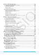
Chapter 19: Performing Data Communication................................................................ 285 19-1 Data Communication Overview .........................................................................................285 Using the ClassPad Communication Application ................................................................................... 285 Select Connection Mode Dialog Box ......................................................................................................
About This User’s Guide • The four digit boldface example numbers (such as 0201 ) that appear in Chapters 2 through 14 indicate operation examples that can be found in the separate “Examples” booklet. You can use the “Examples” booklet in conjunction with this manual by referring to the applicable example numbers. • In this manual, cursor key operations are indicated as f, c, d, e (1-1 General Guide).
Chapter 1: Basics This chapter provides a general overview of the ClassPad and application operations, as well as information about input operations, the handling of data (variables and folders), file operations, and how to configure application format settings. 1-1 General Guide ClassPad at a Glance 3-pin data communication port See Chapter 19 for details. 4-pin mini USB port See Chapter 19 for details. Touch screen Stylus Icon panel See “1-3 Built-in Application Basic Operations”.
Turning Power On or Off While the ClassPad is turned off, press c to turn it on. To turn off the ClassPad, press f and then c. Auto Power Off The ClassPad also has an Auto Power Off feature. This feature automatically turns the ClassPad off when it is idle for a specified amount of time. For details, see “To configure power properties” on page 282. Note Any temporary information in ClassPad RAM (graphs drawn on an application’s graph window, a dialog box displayed, etc.
1-3 Built-in Application Basic Operations This section explains basic information and operations that are common to all of the built-in applications. Using the Application Menu Tapping m on the icon panel displays the application menu. You can perform the operations below with the application menu. Tap a button to start up an application. See “Built-in Applications” below. Tap here (or tap s on the icon panel) to display the next menu. VCP file operations. See page 289. Starts touch panel alignment.
Tap this icon: To start this application: To perform this type of operation: Picture Plot • Plot points (that represent coordinates) on a photograph, illustration, or other graphic and perform various types of analysis based on the plotted data (coordinate values) Interactive Differential Calculus • Learn about the differential coefficients and/or derivative formulas that are the foundation of differentiation Conics • Draw the graph of a conics section Differential Equation Graph • Draw vector fie
Application Window The following shows the basic configuration of a built-in application window. Menu bar Tool bar Upper window Application window(s) Lower window Soft keyboard See page 18. Status bar See page 17. Many applications split the display between an upper window and a lower window, each of which shows different information. When using two windows, the currently selected window (the one where you can perform operations) is called the “active window”.
Using the O Menu The O menu appears at the top left of the window of each application, except for the System application. You can access the O menu by tapping m on the icon panel, or by tapping the menu bar’s O menu. The following describes all of the items that appear on the O menu. 1 Tapping [Variable Manager] starts up Variable Manager. See “Using Variable Manager” (page 29) for details. 1 2 2 Tapping [View Window] displays a dialog box for configuring the display range and other graph settings.
u To terminate an operation Pressing the c key while an expression processing, graphing, or other operation is being performed terminates the operation and displays a “Break” dialog box like the one shown nearby. Tap the [OK] button on the dialog box to exit the Break state. 1-4 Input You can input data on the ClassPad using its keypad or by using the on-screen soft keyboard. Virtually all data input required by your ClassPad can be performed using the soft keyboard.
Trig Advance For details above the above key sets, see “Using Math, Trig, and Advance Key Sets” (page 23). [Var] (variable) key set This key set includes only keys for the input of single-character variables. For more information, see “Using Single-character Variables” (page 25). [abc] key set Use this key set to input alphabetic characters. Tap one of the tabs along the top of the keyboard (along the right when using horizontal display orientation) to see additional characters, for example, tap [Math].
k Inputting a Calculation Expression You can input a calculation expression just as it is written, and press the E key to execute it. The ClassPad automatically determines the priority sequence of addition, subtraction, multiplication, division, and parenthetical expressions. Example: To simplify −2 + 3 − 4 + 10 u Using the keypad keys cz2+3-4+10E If the line where you want to input the calculation expression already contains input, be sure to press c to clear it.
Example: To change 302 to sin(30)2 (For input, use the keypad and the [Math1] soft keyboard set.) 1. c30x 2. dddds 3. ee) u To replace a range of input with new input After you drag the stylus across the range of input that you want to replace, enter the new input. Example: To change “1234567” to “10567” 1. c1234567 2. Drag the stylus across “234” to select it. 3.
k Copying with Drag and Drop You can also copy a string of text by simply selecting it and then dragging it to another location that allows text input. Example 1: To use the Main application to perform the calculation 15 + 6 × 2, edit to (15 + 6) × 2, and then re-calculate 1. In the Main application work area, perform the calculation below. c15+6*2E 2. Drag across the 15 + 6 × 2 expression to select it, and then drag the expression to the . • This will copy 15 + 6 × 2 to the location where you dropped it.
k Using Math, Trig, and Advance Key Sets The [Math1], [Math2], [Math3], [Trig] (trigonometric), and [Advance] key sets contain keys for inputting numeric expressions. The L key in the upper left corner and all of the keys in the bottom row are common to all key sets. Their functions are described below. L Switches between template input and line input. See “Template Input and Line Input” (page 24). h Performs the same operation as the keypad’s K key.
Key set Key Description Math2 `*7 ]_) “Using the Calculation Submenu” (page 67) Math2 678 “2-5 Matrix and Vector Calculations” (page 58) Math3 d Math3 fg Math3 ' “Derivative Symbol (’)” (page 54) Math3 + “dSolve [Action][Equation/Inequality][dSolve]” (page 82) Math3 1 “piecewise Function” (page 54) Math3 U “with Operator ( | )” (page 55) Math3 [ Inputs square brackets ([ ]).
u Switching between Template Input and Line Input Tap the L key. Each toggles the key color between white (L) and light blue ( ). A white key indicates the template input mode, while a light blue key indicates the line input mode. In the template input mode, you can perform template input using keys with or marked on their key tops, such as N and !. Other keys input the same functions or commands as they do in the line mode. 2' 2 ' 2 + 1 1.
u To input a single-character variable name Any character you input using any one of the following techniques is always treated as a single-character variable. • Tapping any key in the [Var] (variable) key set (page 19) • Tapping the X, Y, or Z key of the [Number] key set • Tapping the [ key of the [Math2] key set • Pressing the x, y, or Z keypad key If you use the above key operations to input a series of characters, each one is treated as a single-character variable.
k Using the Catalog Keyboard The “Form” menu of the catalog keyboard lets you select one of the five categories described below. Func ........ built-in functions (pages 48 and 61) Cmd ........ built-in commands and operators (page 206) Sys .......... system variables (page 299) User ........ user-defined functions (page 203) All ............ all commands, functions, etc. After selecting a category, you can choose the item you want from the alphabetized list that appears on the catalog keyboard.
• Saving a spreadsheet to a file (by executing [File] - [Save] with the Spreadsheet application) saves the file in main memory as “MEM” (memory) type data. An eActivity file created with the eActivity is stored in a separate eActivity memory area in order to keep it separate from other application data. Accessing Data Besides the application that originally created it, data in main memory can also be accessed by any other application.
User folder: This is a folder created and named by you. You can make a user folder the current folder, move data to a user folder, etc. You can also delete and rename a user folder as required. You can have up to 87 user folders in main memory at one time. Tip: You cannot put a folder inside of another folder. Current Folder The current folder is the folder where the data (excluding eActivity files) created by applications are stored and from which such data can be accessed.
u Variable Manager operations The operations described in the table below can be performed while Variable Manager is displayed. To do this: Do this: Specify the current folder On the folder list, tap the [Current] down arrow button. On the list that appears, select the folder that you want to specify as the current folder. Create a folder On the folder list, tap [Edit] - [Create Folder]. On the dialog box that appears, enter the name you want to assign to the folder and then tap [OK].
Selecting a Folder • If no check box is selected on the folder list, any folder operation that is performed affects the folder whose name is currently highlighted on the list. If any folder check box is selected, only that folder is affected by a folder operation, and the folder whose name is highlighted on the list is not affected. • Selecting the check box of a folder causes the check boxes of all of the variables inside of it also to become selected.
4. Tap the folder or variable whose name you want to input, so its name is highlighted. 5. Tap [INPUT]. • This exits Variable Manager and inputs the name of the folder or variable you selected in step 4 into the application at the current cursor position. Managing Application Files The applications below can save data to files.
u To rename a folder or file 1. Tap [File] and then [Open]. 2. On the dialog box that appears, tap the name of the folder or file you want to rename so it is selected. 3. Tap [File] and then [Rename]. This displays the Rename dialog box. 4. Enter the name you want to assign to it and then tap [OK]. u To move a file to another folder 1. Tap [File] and then [Open]. 2. On the dialog box that appears, select the check box next to the file you want to move.
• This creates a variable named “eq1” in the current folder (the “main” folder in this example), and assigns the expression 2x + 1 to it. Tip • If a variable with the specified name already exists in the current folder, the contents of the existing variable are replaced with the newly assigned data, unless the existing variable is locked or protected. For more information, see “Variable Manager operations” (page 30) and “Protected variable types” (page 28).
4. Change the current folder specification to “Test”. • Use Variable Manager (page 29) to create a folder named “Test” and change the current folder specification. 5. Perform the following operations to view the contents of variables “eq1” and “eq2”. eq1E (Since this key operation does not access the “main” folder, the variable name (“eq1”) is displayed without showing the variable contents.) main\eq1E (Specifying the path to the “main” folder where “eq1” is located displays the contents of the variable.
1-7 Configuring Application Format Settings The O menu includes format settings for configuring the number of calculation result display digits and the angle unit, as well as application-specific commands. The following describes each of the settings and commands that are available on the O menu.
To do this: Do this: Switch between complex number calculations (Complex mode) and real number calculations (Real mode) Select the “Complex Format” check box to enter the Complex mode, or clear the check box* to enter the Real mode*. Display results as a decimal value (Decimal mode) or leave calculation results as expressions (Standard mode) Select the “Decimal Calculation” check box to enter the Decimal mode, or clear the check box* to enter the Standard mode.
k Graph Format Dialog Box Use the Graph Format dialog box to configure settings for the Graph window and for drawing graphs. [Basic] tab 1 2 3 4 To specify display of Graph window axes Tap 1 and then tap one of the settings described below. On: show axis Off: hide axis Number*: show axis along with maximum and minimum value of each axis To specify display of Graph window grid Tap 2 and then tap one of the settings described below.
[Special] tab 1 2 3 To specify the row width for Stat Editor and data table displays Tap 1 and then select a cell width pattern: 2 Cells, 3 Cells*, or 4 Cells for vertical display orientation, or 4 Cells, 5 Cells*, or 6 Cells for horizontal orientation (see “Changing the Display Orientation” on page 16). To specify a source for table data Tap 2 and then tap one of the settings described below. Table Input*: Uses the data input in a Table Input dialog box as the source for number table generation.
k Geometry Format Dialog Box Use the Geometry Format dialog box to configure settings for the Geometry application. Tip: The information that appears in the preview area at the bottom of the dialog box shows a preview of the Geometry application window, based on the settings configured in upper part of the dialog box. 1 2 3 4 5 6 To specify the Geometry window numeric value display format Tap 1 and then select the format you want. The initial default Number Format setting is Fix2.
k Financial Format Dialog Box Use the Financial Format dialog box to configure settings for the Financial application. [Basic] tab To specify the number of days in a year Tap 1, and then tap “360 days” or “365 days*”. 1 2 3 To specify the beginning or the period or the end of the period as the payment date Tap 2 and then tap “Beginning of period” or “End of period*”. To specify the date format Tap 3 and then tap one of the settings described below.
[Special] tab 1 2 3 4 5 To specify odd period handling Tap 1 and then tap one of the settings described below.
1-8 When you keep having problems… If you keep having problems when you are trying to perform operations, try the following before assuming that there is something wrong with the ClassPad. 1. Initialize all application format settings. Perform the procedure under “Initializing All Application Format Settings” (page 42). 2. Perform the RAM reset (RESTART) operation. Perform RAM reset when the ClassPad freezes up or otherwise fails to perform as expected for some reason.
Chapter 2: Main Application The Main application is a general-purpose numerical and mathematical calculation application that you can use to study mathematics and solve mathematical problems. You can use the Main application to perform general operations from basic arithmetic calculations, to calculations that involve lists, matrices, etc. Starting up the Main application displays a large white work area. Use this area for inputting operations and commands.
• All of the example calculations shown in 0201 are performed using the keypad or the soft keyboard [Number] key set, unless noted otherwise. • The example calculations are all performed using the Decimal mode (page 46). Using the e Key Use the e key to input exponential values. You can also input exponential values using the E key on the soft keyboard [Number] key set. 0202 Calculation examples Omitting the Multiplication Sign You can omit the multiplication sign in any of the following cases.
Calculation Priority Sequence Your ClassPad automatically performs calculations in the following sequence. 1 Commands with parentheses (sin(, diff(, etc.) 5 +, –, (–) 2 Factorials (x!), degree specifications (o, r ), percents (%) 6 Relational operators (=, , <, >, s, t) 7 and 3 Powers 4 π, memory, variable multiplication operations that omit the multiplication sign (2π, 5A, etc.), command with parentheses multiplication operations that omit the multiplication sign (2' 3, etc.
u Number of Decimal Places, Number of Significant Digits, Normal Display Settings The [Number Format] settings on the Basic Format dialog box specify the number of decimal places, the number of significant digits, and the normal display setting for Main application Decimal mode calculation results. The following shows how calculation results appear under each setting. Expression Normal 1 Normal 2 Fix 3 Sci 3 12.5 12.5 12.500 1.25E + 1 100 ÷ 6 = 16.6666666... 16.66666667 16.66666667 16.667 1.
2-2 Using the Calculation History The Main application work area calculation history can contain up to 30 expression/result pairs. You can look up a previous calculation, edit, and then re-calculate it, if you want. • Use the scroll bar or scroll buttons to scroll the work area window up and down. This brings current calculation history contents into view. • You can edit a calculation expression in the calculation history and then re-calculate the resulting expression.
Problem Operation Convert 4.25 radians to degrees. = 243.5070629 4.25 Rw 47.3° + 82.5rad = 4774.20181° 47.3 + 82.5 Rw How many radians is 243.5070629°? = 4.249999999 Change the [Angle] setting to “Radian”, and then input 243.5070629 *w. Trigonometric and Inverse Trigonometric Functions Problem Operation cos(( π ) rad) = 0.5 3 Change the [Angle] setting to “Radian”. 2 · sin45° × cos65° = 0.5976724775 Change the [Angle] setting to “Degree”. 2*s 45 )*c 65 w c7/ 3 w or cN7c 3 w Can be omitted.
Other Functions (%, ', x2, x –1, x!, abs, ⬔, signum, int, frac, intg, fRound, sRound) Problem What is 12% of 1500? Operation 1500 * 12 &w (180) What percent of 880 is 660? 660 / 880 &w (75%) What value is 15% greater than 2500? What value is 25% less than 3500? (2875) (2625) ' 2+' 5 = 3.65028154 2500 *( 1 + 15 & 3500 *( 1 - 25 & 5 2 e+5 5 w (3 + i) = 1.755317302 + 0.2848487846i Change to the Complex mode (“Cplx” indicated on the status bar).
u “rand” Function The “rand” function generates random numbers. If you do not specify an argument, “rand” generates 10-digit decimal values 0 or greater and less than 1. Specifying two integer values for the argument generates random numbers between them. Problem Operation Generate random numbers between 0 and 1. [rand] w Generate random integers between 1 and 6.
Function: • Omitting a value for “m” (or specifying 1 for “m”) returns the generated random number as-is. • Specifying 2 or larger value for “m” returns the specified number of random values in list format. Description: • “n” and “m” must be positive integers. Problem Operation Randomly produce the number of heads that can be expected in accordance with binomial distribution for five coin tosses where the probability of heads is 0.5. [randBin] 5 , 0.
Problem Operation Determine the greatest common divisors of {4, 3}, {12, 6}, and {36, 9}. [iGcd] { 4 , 3 },{ 12 , 6 },{ 36 , 9 })w u “iLcm” Function Syntax: iLcm(Exp-1, Exp-2[, Exp-3…Exp-10)] (Exp-1 through Exp-10 all are integers.) iLcm(List-1, List-2[, List-3…List-10)] (All elements of List-1 through List-10 are integers.) Function: • The first syntax above returns the least common multiple for two to ten integers.
Condition Judgment (judge, piecewise) u “judge” Function The “judge” function returns TRUE when an expression is true, and FALSE when it is false. Problem Operation Is the following expression true or false? 1=1 TRUE [judge] 1 = 1 w Is the following expression true or false? 1<0 FALSE [judge] 1 < 0 w u “piecewise” Function The “piecewise” function returns one value when an expression is true, and another value when the expression is false. The syntax of the “piecewise” function is shown below.
Primality Test (isPrime) The “isPrime” function determines whether the number provided as the argument is prime (returns TRUE) or not (returns FALSE). The syntax of the “isPrime” function is shown below. isPrime(Exp/List[ ) ] • Exp or all of the elements of List must be integers. Problem Operation Determine whether the numbers 51 and 17 are prime.
Solutions Supported by ClassPad (TRUE, FALSE, Undefined, No Solution, ∞, const, constn) Solution Description Example TRUE Output when a solution is true. judge (1 = 1) w FALSE Output when a solution is false. judge (1 < 0) w Undefined Output when a solution is undefined. 1/0 w No Solution Output when there is no solution. solve (abs (x) = –1, x) w ∞ Infinity lim (1/x2, x, 0) w const Constant displayed as const(1) when any value that is a constant is included in the solution.
Gamma Function The Gamma function is called “gamma” on the ClassPad. +∞ ∫0 Γ(x) = t x–1e–t dt For an integer n the gamma is evaluated as shown below. Q ² Q ! ^ XQGHILQHG Q s KQ The gamma is defined for all real numbers excluding zero and negative integers. It is also defined for all complex numbers where either the real or imaginary part of the complex number is not an integer. Gamma of a symbolic expression returns unevaluated.
2-5 Matrix and Vector Calculations This section explains how to create matrices, and how to perform basic matrix calculations. Tip: Since a vector can be viewed as 1-row by n-column matrix or n-row by 1-column matrix, this section does not include explanations specifically about vectors. For more information about vector-specific calculations, see the explanations about the applicable [Action] menu items in “2-7 Using the Action Menu”.
Raising a Matrix to a Specific Power Example: To raise 1 3 2 4 to the power of 3 0226 Input in a single line 0227 Input using an actual on-screen matrix Tip: You can raise only a square matrix to a specific power. An error occurs when you try to raise a non-square matrix to a specific power. Using a Matrix to Assign Different Values to Multiple Variables Use the procedure in this section when you want to use a matrix to assign various different values to multiple variables.
Selecting a Number Base Specifying a default number base in the Main application will apply to the current line (expression/result pair), and to all subsequent lines until you change the default number base setting. u To select the number base for the line where the cursor is located 1. Tap the down arrow button next to the < button. 2. Tap the button that corresponds to the number base you want to use: 1 (binary), 2 (octal), 3 (decimal), 4 (hexadecimal).
Using the baseConvert Function (Number System Transform) The baseConvert function lets you convert a number in one base (number system) to its equivalent in another base. Important! • The baseConvert function works for positive integers only. • The baseConvert function cannot be used in a line for which a particular number base is specified. It can be used in a normal calculation line only.
Example Screenshots The screenshots below show examples of how input and output expressions appear on the ClassPad display. All of the screenshots in this section show the “complete expression” version. When the input expression does not fit: Displayed expression Complete expression When the output expression does not fit: Displayed expression Complete expression Using the Transformation Submenu The [Transformation] submenu contains commands for expression transformation, like “expand” and “factor”.
u rFactor [Action][Transformation][factor][rFactor] Function: Factors an expression up to its roots, if any. Syntax: rFactor (Exp/Eq/Ineq/List/Mat [ ) ] Example: To factor x2 3 u factorOut [Action][Transformation][factor][factorOut] Function: Factors out an expression with respect to a specified factor.
u toFrac [Action][Transformation][Fraction][toFrac] Function: Transforms a decimal value into its equivalent fraction value. Syntax: toFrac (Exp/Eq/Ineq/List/Mat [ ) ] Example: To transform 5.28 into its equivalent fraction value u propFrac [Action][Transformation][Fraction][propFrac] Function: Transforms a decimal value into its equivalent proper fraction value. Syntax: propFrac (Exp/Eq/Ineq/List/Mat [ ) ] Example: To transform 1.
Syntax: laplace( f (t), t, s) invLaplace(L(s), s, t) f (t): expression ; t: variable with respect to which the expression is L(s): expression ; s: variable with respect to which the expression is transformed ; transformed ; s: parameter of the transform t: parameter of the transform ClassPad supports transform of the following functions. x, ex, heaviside(x), delta(x), delta(x, n) sin(x), cos(x), sinh(x), cosh(x), xn, ' ClassPad does not support transform of the following functions.
To restore the symmetry of the transforms, the convention shown below is sometimes used. ( ) = [ ( )] = ∞ 1 ∫–∞ 2π ( ) – ( ) = –1[ ( )] = ∞ 1 2π ∫–∞ ( ) In general, the Fourier transform pair may be defined using two arbitrary constants a and b as shown below.
Using the Calculation Submenu The [Calculation] submenu contains calculus related commands, such as “diff” (differentiation) and “ ” (integration). u diff [Action][Calculation][diff] Function: Differentiates an expression with respect to a specific variable. Syntax: diff(Exp/List[,variable] [ ) ] diff(Exp/List,variable,order[,a] [ ) ] • “a” is the point for which you want to determine the derivative. • “order” = 1 when you use the following syntax: diff(Exp/List[,variable][ ) ].
u Σ [Action][Calculation][Σ] Function: Evaluates an expression at discrete variable values within a range, and then calculates a sum. Syntax: Σ(Exp/List, variable, lower value, upper value [ ) ] Example: To calculate the sum of x2 as the value of x changes from x = 1 through x =10 u Π [Action][Calculation][Π] Function: Evaluates an expression at discrete variable values within a range, and then calculates a product.
u fMin [Action][Calculation][fMin/fMax][fMin], fMax [Action][Calculation][fMin/fMax][fMax] Function: Returns the minimum (fMin) / the maximum (fMax) point in a specific range of a function. Syntax: fMin(Exp[,variable] [ ) ] fMin(Exp, variable, start value, end value[,n] [ ) ] fMax(Exp[,variable] [ ) ] fMax(Exp, variable, start value, end value[,n] [ ) ] • “x” is the default when you omit “[,variable]”.
Using the Complex Submenu The [Complex] submenu contains commands that relate to calculations that involve complex numbers. u arg [Action][Complex][arg] Function: Returns the argument of a complex number. Syntax: arg (Exp/Eq/List/Mat [ ) ] Example: To obtain the argument of complex 2 + i (in the Radian mode) u conjg [Action][Complex][conjg] Function: Returns the conjugate complex number.
u compToRect [Action][Complex][compToRect] Function: Transforms a complex number into its rectangular form. Syntax: compToRect (⬔(r, ) or r · e^( · i) form [ ) ] Example: To transform a complex number into its rectangular form Using the List-Create Submenu The [List][Create] submenu contains commands that are related to creating lists. u seq [Action][List][Create][seq] Function: Generates a list in accordance with a numeric sequence expression.
u rotate [Action][List][Create][rotate] Function: Returns a list in which the elements have been rotated to the right or to the left by a specific amount. Syntax: rotate (List [,number of rotations] [ ) ] • Specifying a negative value for “[,number of rotations]” rotates to the right, while a positive value rotates to the left. Example: To rotate the elements of the list {1, 2, 3, 4, 5, 6} to the left by two • Right rotation by one (–1) is the default when you omit “[,number of rotations]”.
u median [Action][List][Statistics][median] Function: Returns the median of the elements in a list. Syntax: median (List-1[, List-2] [ ) ] (List-1: Data, List-2: Freq) Example: To determine the median of the elements in the list {1, 2, 3} u mode [Action][List][Statistics][mode] Function: Returns the mode of the elements in a list. If there are multiple modes, they are returned in a list.
u prod [Action][List][Calculation][prod] Function: Returns the product of the elements in a list. Syntax: prod (List-1[, List-2] [ ) ] (List-1: Data, List-2: Freq) Example: To determine the product of the elements in the list {1, 2, 3} u cuml [Action][List][Calculation][cuml] Function: Returns the cumulative sums of the elements in a list.
Syntax: sumSeq (List-1[, List-2] [,variable] [ ) ] • “x” is the default when you omit “[,variable]”. Example: To determine the sum of a polynomial for a sequence expressed by the list {3, 5, 7, 9} Using the Matrix-Create Submenu The [Matrix][Create] submenu contains commands related to creation of matrices. u trn [Action][Matrix][Create][trn] Function: Returns a transposed matrix.
u listToMat [Action][Matrix][Create][listToMat] • For information about listToMat, see page 72. u matToList [Action][Matrix][Create][matToList] Function: Transforms a specific column of a matrix into a list. Syntax: matToList (Mat, column number [ ) ] Example: To transform column 2 of the matrix [[1, 2] [3, 4]] into a list Using the Matrix-Calculation and Matrix-Row&Column Submenus The [Matrix][Calculation] and [Matrix][Row&Column] submenus contain commands that are related to matrix calculations.
u eigVl [Action][Matrix][Calculation][eigVl] Function: Returns a list that contains the eigenvalue(s) of a square matrix. Syntax: eigVl (Mat [ ) ] Example: To obtain the eigenvalue(s) of the matrix [[3, 4] [1, 3]] u eigVc [Action][Matrix][Calculation][eigVc] Function: Returns a matrix in which each column represents an eigenvector of a square matrix. • Since an eigenvector usually cannot be determined uniquely, it is standardized as follows to its norm, which is 1: When V = [x1, x2, ...
u mRow [Action][Matrix][Row&Column][mRow] Function: Multiplies the elements of a specific row in a matrix by a specific expression. Syntax: mRow (Exp, Mat, row number [ ) ] Example: To multiply row 1 of the matrix [[1, 2] [3, 4]] by x u mRowAdd [Action][Matrix][Row&Column][mRowAdd] Function: Multiplies the elements of a specific row in a matrix by a specific expression, and then adds the result to another row.
Using the Vector Submenu The [Vector] submenu contains commands that are related to vector calculations. • A vector is handled as a 1 × N matrix or N × 1 matrix. • A vector in the form of 1 × N can be entered as [……] or [[……]]. Example: [1, 2], [[1, 2]] • Vectors are considered to be in rectangular form unless ∠() is used to indicate an angle measure. u augment [Action][Vector][augment] Function: Returns an augmented vector [Mat-1 Mat-2].
u norm [Action][Vector][norm] Function: Returns the norm of a vector. Syntax: norm (Mat [ ) ] Example: To obtain the norm of the vector [1, 2, 3] u crossP [Action][Vector][crossP] Function: Returns the cross product of two vectors. Syntax: crossP (Mat-1, Mat-2 [ ) ] • This command can be used with a 1 × N or N × 1 matrix only (N = 2, 3). • A two-element matrix [a, b] or [[a], [b]] is automatically converted into a three-element matrix [a, b, 0] or [[a], [b], [0]].
Example: To transform the rectangular form [1, 1, 1] into its equivalent spherical form (in the Radian mode) u toCyl [Action][Vector][toCyl] Function: Returns an equivalent cylindrical form [r∠ z]. Syntax: toCyl (Mat [,natural number] [ ) ] • This command can be used with a 1 × 3 or 3 × 1 matrix only. • This command returns “r” when “natural number” is 1, “ ” when “natural number” is 2, and “z” when “natural number” is 3. • This command returns a cylindrical form when you omit “natural number”.
Syntax 4: You can solve for the relationship between two points, straight lines, planes, or spheres by entering a vector equation inside the solve( command. Here we will present four typical syntaxes for solving a vector equation using the solve( command. In the syntaxes below, Vct-1 through Vct-6 are column vectors with three (or two) elements, and s, t, u and v are parameters.
u rewrite [Action][Equation/Inequality][rewrite] Function: Moves the right side elements of an equation or inequality to the left side. Syntax: rewrite(Eq/Ineq/List [ ) ] Example: To move the right side elements of x + 3 = 5x – x2 to the left side u exchange [Action][Equation/Inequality][exchange] Function: Swaps the right-side and left-side elements of an equation or inequality.
u or [Action][Equation/Inequality][Logic][or] Function: Returns the result of the logical OR of two expressions. Syntax: Exp/Eq/Ineq/List-1 or Exp/Eq/Ineq/List-2 Example: To obtain the result of the logical OR of x = 3 or x > 2 u xor [Action][Equation/Inequality][Logic][xor] Function: Returns the logical exclusive OR of two expressions.
Using the Distribution/Inv.Dist Submenu The [Distribution/Inv.Dist] submenu includes functions related to each type of statistical calculation distribution probability. The functions on this submenu perform the same calculations as the Distribution commands that are available in the Statistics application and the Main, eActivity, and Program applications. For information about the numeric expressions used in calculations, see “Distributions” on page 151.
u normCDf [Action][Distribution/Inv.Dist][Continuous][normCDf] Function: Returns the cumulative probability of a normal distribution between a lower bound and an upper bound. Syntax: normCDf(lower value, upper value[,σ , μ)] • When σ and μ are skipped, σ = 1 and μ = 0 are used. Calculation Result Output: prob, zLow, zUp Example: To determine the normal probability density when lower bound value = −∞, upper bound value = 36, σ = 2, μ = 35 u invNormCDf [Action][Distribution/Inv.
u invTCDf [Action][Distribution/Inv.Dist][Inverse][invTCDf] Function: Returns the lower bound value of a Student’s t cumulative distribution probability for specified values. Syntax: invTCDf(prob, df [ ) ] Calculation Result Output: xInv Example: To determine the lower bound value when prob = 0.0754752, df = 18 u chiPDf [Action][Distribution/Inv.Dist][Continuous][chiPDf] Function: Returns the χ2 probability density for specified values.
u invFCDf [Action][Distribution/Inv.Dist][Inverse][invFCDf] Function: Returns the lower bound value of an F cumulative distribution probability for specified values. Syntax: invFCDf(prob, n:df, d:df [ ) ] Calculation Result Output: xInv Example: To determine the lower bound value when prob = 0.1852, n:df = 24, d:df = 19 u binomialPDf [Action][Distribution/Inv.Dist][Discrete][binomialPDf] Function: Returns the probability in a binomial distribution that the success will occur on a specified trial.
u poissonCDf [Action][Distribution/Inv.Dist][Discrete][poissonCDf] Function: Returns the cumulative probability in a Poisson distribution that the success will occur between specified lower value and upper value. Syntax: poissonCDf(lower value, upper value, [ ) ] Calculation Result Output: prob Example: To determine the Poisson cumulative probability when lower value = 2, upper value = 3, = 2.26 u invPoissonCDf [Action][Distribution/Inv.
u hypergeoPDf [Action][Distribution/Inv.Dist][Discrete][hypergeoPDf] Function: Returns the probability in a hypergeometric distribution that the success will occur on a specified trial. Syntax: hypergeoPDf(x, n, M, N [ ) ] Calculation Result Output: prob Example: Determine the hypergeometric probability when x = 1, n = 5, M = 10, N = 20. u hypergeoCDf [Action][Distribution/Inv.
u Clear_a_z Function: Clears all single-character variables. For more information, see “Clear_a_z” on page 84. u DelVar Function: Deletes a specified variable. For more information, see “DelVar” on page 208. u Clear All Variables Function: Clear variables that contain numbers, list and matrices. 2-8 Using the Interactive Menu The [Interactive] menu includes most of the commands that are on the [Action] menu. Selecting a command on the [Action] menu will simply input the command.
2-9 Using the Main Application in Combination with Other Applications You can access the windows of other ClassPad applications from the Main application and perform copy, paste, drag and drop, and other operations between them. Tip • Copying data that includes color information from another application and pasting it into the Main application will cause the color information to be disregarded, and the pasted data will become black.
• As can be seen in this example, a graph can be drawn by dropping an expression in the form of f (x) into the Graph window. • When dropping a formula into the 3D Graph window instead of the Graph window, the formula must be in form f (x, y) (such as x^2+y^2). Using the Stat Editor Window You can use the Stat Editor window to create new LIST variables and edit existing LIST variables. You can also use the Stat Editor window to specify a LIST variable’s name and display its contents.
Tip: The following shows what happens when you drag a figure from the Geometry window to the work area.
2-11 Using Probability You can use Probability to simulate the following.
2-12 Running a Program in the Main Application You can run a program in the Main application or the eActivity application. Syntax: Folder name\Program name(parameter) • You do not need to specify the folder name if the program you want to run is in the current folder. If you leave ClassPad configured with its initial default settings, the current folder for both the Program application and the Main application is the “main” folder, so you normally do not need to specify a folder name.
Chapter 3: Graph & Table Application The Graph & Table application allows you to input and graph rectangular coordinate equations (or inequalities), polar coordinate equations, and parametric expressions. After you graph an expression, you can perform various graph-based analytical operations, such as determining the points of intersection of two graphs, point of inflection, and definite integral for a particular range of a parabola or other figure.
• Graph the selected function(s) ....................................................................................................................$ • Generate a summary table for the selected function ..................................................................................4 • Display the View Window dialog box to configure Graph window settings .................................................6 • Display the Table Input dialog box for configuring settings........................................
3-1 Storing Functions Use the Graph Editor window to store a Graph & Table application function. This section covers Graph Editor operations, and explains how to store functions. Using Graph Editor Sheets The Graph Editor window has five tabbed sheets named Sheet 1 through Sheet 5, each of which can contain up to 20 functions. You can graph up to 20 functions simultaneously, as long as all of the functions are on the same sheet. The table below explains Graph Editor sheet operations.
To input this type of expression: Do this: x equality 1. Tap [Type] - [x=Type]. 2. Input an expression that includes variable y and then press E. y inequality (left side y type) 1. Tap [Type], [Inequality], and then tap one of the following: [y>Type], [yType], [x
2. Configure the dialog box with the following settings. To specify this: Perform this operation: Line type Tap “Graph Plot” and then tap the desired line type. Line color Tap “Line Color” and then tap the desired color. 3. To apply the settings, return to the dialog box in step 2 of this procedure and then tap [OK].
Saving Graph Editor Data to Graph Memory Graph memory lets you store all of the expressions and their related information to a file for later recall.
2. If you want to configure settings using preset ClassPad View Window parameters, perform the operations described below. To configure this setting: Do this: ClassPad initial defaults On the [Memory] menu select [Initial], or tap the [Default] button. Configure settings optimized for trigonometric function graphing On the [Memory] menu, select [Trigonometric]. Display both the x-axis and y-axis in a range of –10 to 10 On the [Memory] menu, select [Standard].
Parameter Name Description Trigonometric • xscale is set to π/2* radian = 90 degree = 100 grad. The values depend on the Basic Format Angle setting. This xscale is used as the basis to display an x-axis direction in the range of xscale × –7.7 (xmin) to xscale × 7.7 (xmax). For example, when the Angle setting is Degree, xmin = –693, xmax = 693. • y-axis settings are fixed as follows, regardless of the Angle setting: yscale = 1, ymin = –2.1, ymax = 2.1.
Tip • Graph window panning cannot be performed while any one of the following functions is being used: Modify, Trace, Sketch, G-Solve, box zoom. • While a panning operation is in progress on the Graph window, the coordinates of the point where the stylus is held against the display is displayed in the status bar. Scrolling the Graph Window You can use either of the two operations to scroll the Graph window up, down, left, or right. • Tapping the graph controller arrows at the edges of the Graph window.
Using Quick Zoom The quick zoom commands on the [Zoom] menu draw a graph using preset built-in View Window parameter values. Note • The values in the explanations below apply during the vertical half-size view of the Graph window (which is the initial default setting of the Graph & Table application). Tapping r on the icon panel will switch to the full-screen view and change the View Window settings.
Saving a Screenshot of a Graph Use the following procedures to save a screenshot of a graph as image data for later recall. u To open a screenshot of a graph 1. On the Graph window, tap a and then [Open Picture]. This displays a list of names of graph images you have stored in memory. 2. Select the name of the image you want, and then tap [OK]. • The image you select is displayed as the Graph window background. u To save a screenshot of a graph 1. Draw the graph you want to save. 2.
3-3 Using Table & Graph The Graph & Table application includes a “Table window” for displaying number tables and summary tables generated with the functions you input on the Graph Editor window. Generating a Number Table A number table can be created for one or more y=Type, r=Type, or ParamType (Parametric Type) functions registered on the Graph Editor window.
u To generate a number table by assigning list values to x, , or t 1. Tap O and then [Graph Format] to display the Graph Format dialog box. 2. Tap [Special] tab, and then select a list option (list1 through list6 or a list variable created by you) for the [Table Variable] item. • By way of example, here we will select “list1”. 3. Tap [Set] to apply the settings and close the dialog box. 4. Tap O, [Window] and then [Stat Editor] to display the Stat Editor window. 5.
Generating Number Table Values from a Graph You can input the coordinate values where the pointer is currently located on a graph into a table by simply pressing E. 0303 To generate number table values from the y = x3 – 3x graph Generating a Summary Table A summary table can be created from a y=Type function registered on the Graph Editor window. The figure below shows an example of the summary graph and table of y = x3 – 3x.
4. Tap [OK] to close the View Window dialog box. • Tapping $ here graphs the function using the View Window settings. 5. Tap 4. • This starts summary table generation, and displays the result on the Table window. Note that generation of a summary table can take a bit of time. Tip • The above operation is possible only when “View Window” (which is the initial default) is selected for the Graph Format dialog box [Summary Table] item.
2. Tap [Analysis], [Trace], or tap =. • This will display the pointer at the coordinates where x = 0. The pointer will not be visible when it is located at a point outside the graph display area. • If “Undefined” appears in place of the xc or yc coordinate, it means that the current point is undefined. Press the left or right cursor key to move to a point that is defined. 3. Press the left or right cursor key, or tap the left or right graph controller arrow.
u To write text on the Graph window 1. While the Graph window is active, tap [Analysis], [Sketch], and then [Text]. 2. On the dialog box that appears, enter the text you want and then tap [OK]. • This displays the word “Text” in the lower right corner of the Graph window. 3. Place the stylus on the screen and hold it there. • This causes the text you input in step 2 to appear at the location where you are pointing with the stylus. 4.
3-6 Analyzing a Function Used to Draw a Graph Your ClassPad includes a G-Solve feature that lets you perform a variety of different analytical processes on an existing graph. What You Can Do Using the G-Solve Menu Commands While there is a graph on the Graph window, you can use a [G-Solve] menu command to obtain the following information. • x-coordinate for a given y-coordinate .................................................
3. To obtain other roots, press the left or right cursor key, or tap the left or right graph controller arrows. • If there is only one solution, the pointer does not move when you press the cursor key or tap the graph controller arrow. The following are examples for other G-Solve commands.
- Input using the soft keyboard and keyboard (1) Display the soft keyboard and use it to perform the key operation below. a*x{c-b*xw (2) Tap the line below the formula you input and then perform the key operation below. a*x+bw u To run Dynamic Modify 1. On the Graph Editor window, input at least one formula that contains a parameter. 2. Select the check box next to the graph formula(s) you want to use with Dynamic Modify and clear the check boxes of all of the other graphs.
u To exit Dynamic Modify Tap the close button (C) in the upper right corner of the slider display box. Note • While Dynamic Modify is running, up to three sliders can be displayed for the parameters included in the graph formulas whose check boxes are selected. If there are more than three parameters in the selected graph formulas, the three parameters are automatically assigned to sliders in accordance with the rules below.
Chapter 4: Conics Application The Conics application provides you with the capability to graph circular, parabolic, elliptic, and hyperbolic functions. You can also use the Conics application to quickly and easily determine the proper focal point, vertex, directrix, and other information about each type of conics. Starting up the Conics application displays two windows: 1 the Conics Editor window and 2 the Conics Graph window.
4-1 Inputting an Equation You can select one of the preset Conics Forms or input a conics equation manually. You can also transform a manually input equation to a Conics Form. u To input an equation using a Conics Form 1. On the Conics Editor window, tap q to displays the Select Conics Form dialog box. Horizontal Parabola 1 Horizontal Parabola 2 Vertical Parabola 1 Vertical Parabola 2 Circle 1 Circle 2 Ellipse Horizontal Hyperbola Vertical Hyperbola General Form 2.
Drawing a Circle There are two forms that you can use to draw a circle. • One form is the standard form, which allows you to specify the center point and radius: (x – H)2 + (y – K)2 = R2 • The other form is the general form, which allows you to specify the parameters of each term: Ax2 + Ay2 + Bx + Cy + D = 0 Drawing an Ellipse You can use the standard equation ( − H)2 ( − K)2 + = 1 to draw an ellipse. A2 B2 Drawing a Hyperbola A hyperbola can be drawn with either a horizontal or vertical orientation.
Using G-Solve Menu Commands When multiple solutions are obtained by a G-Solve command, only one solution is displayed at a time. For example, executing [Analysis] - [G-Solve] - [Focus] for an ellipse that has two foci will display only one focus at a time. In a case such as this, use the left and right cursor keys (or tap the left and right graph controller arrows) to cycle between the available solutions. u To determine the focus of the parabola x = 2(y – 1)2 – 2 1.
Chapter 5: Differential Equation Graph Application This chapter explains how to use the Differential Equation Graph application, which you can use to investigate families of solutions to ordinary differential equations. The Differential Equation Graph application has the following two types of windows. 1 1 Differential Equation Editor window Use this window to input expressions ([DiffEq] tab) and initial conditions ([IC] tab) for graphing. You also can input f (x) type functions ([Graphs] tab).
• Toggle the use of unit vectors on or off for slope field or phase plane graphing ...............................................................................................................Edit - Unit Vectors • Display the Differential Equation Editor window [DiffEq] tab........................Edit - Editor - DiffEqGraph Editor • Display the Differential Equation Editor window [IC] tab ..............................................
Graphing a Second Order Differential Equation This section explains how to input a second order differential equation, draw a phase plane, and graph the solution curve(s). With this application, a second order differential equation is input in the form of a set of two first order differential equations. • A phase plane is the family of solutions of either a second order differential equation or two first order differential equations of the form x’ = dx/dt = f (x, y) and y’ = dy/dt = g(x, y).
Configuring and Modifying Initial Conditions You can modify an existing initial condition on the Differential Equation Graph window by dragging it. You can also configure a new initial condition on the Differential Equation Graph window by tapping the coordinates you want to specify as the new initial condition. u To modify an initial condition on the Differential Equation Graph window 1.
3. On the Differential Equation Graph window, tap the coordinates that you want to specify as the new initial condition. • This will set the coordinates as the new initial condition and draw a solution curve. • The newly configured initial condition is added to the initial condition editor. To view it, tap the [IC] tab. Configuring Differential Equation Graph View Window Parameters You can set a number of graphing parameters on the View Window dialog box. This dialog box contains two tabs.
Setting Description Solution Dir. A solution curve is graphed starting at the initial condition value t0 and continues until it reaches a target value, which can be either tmin or tmax. The solution direction determines the target values. Forward will graph the solution curve from t0 to tmax. Backward will graph the solution curve from t0 to tmin. Both will graph the solution curve from t0 to tmin, and then t0 to tmax.
u To start a graph/curve trace 1. Draw a solution curve (pages 123 through 124) or function graph (page 127). 2. Tap = or [Analysis] - [Trace]. 5-4 Graphing an Expression or Value by Dropping It into the Differential Equation Graph Window You can use the procedures in this section to graph an expression or value by dragging it from the eActivity application window or the Main application window, and dropping it into the Differential Equation Graph window.
Chapter 6: Sequence Application The Sequence application provides you with the tools you need to work with explicit sequences and recursive type sequences. Starting up the Sequence application displays two windows. 1 Sequence Editor window 1 Use this window to input expressions for creating a sequence table. 2 Table window Use this window to create and display table. (a) Title: Shows the equation used in the calculations. The title is not displayed when an item in column n is selected.
Buttons common to multiple windows • Create an ordered pair table (Editor/Graph/RUN) ......................................................................................# • Create a sequence table with column(s) that determine if a sequence is an arithmetic sequence, geometric sequence, progression of difference, or Fibonacci sequence (Editor/Graph/RUN) ..........................
Determining the General Term of a Recursion Expression You can use the rSolve function to convert the sequence expressed by a recursion expression to the general term format an = f (n). 0602 To determine the general term of the recursion expression an+1 = an + 2, a1 = 1 About rSolve The rSolve function returns the explicit formula of a sequence that is defined in relation to one or two previous terms, or a system of recursive formulas.
Chapter 7: Statistics Application The Statistics application provides you with the tools you need to perform the operations below.
2. Input the data you want. • You can input values, formulas, or variable names. If you input a formula, the value of the calculation result will be input into the list. If you input a variable name, the value currently assigned to the variable (or the variable name itself in the case of an undefined variable) will be input into the list.
• Clear list variable data from list1 through list6 and initialize Stat Editor window contents ..................................................................................................................Edit - Clear All • Convert a mathematical expression in the currently selected cell to a decimal value ................................9 • Display two, three, or four columns in the Stat Editor window*...................................................
u To specify the CSV file separator and decimal symbol 1. While the Stat Editor is on the display, tap [Edit] - [CSV] - [CSV Format]. 2. On the dialog box that appears, specify the desired settings for “CSV Separator” and “CSV Decimal Symbol”. 3. To save the settings, tap [OK]. 7-2 Drawing a Statistical Graph Up to nine graphs, including single-variable data and paired-variable data statistical graphs can be drawn simultaneously ([SetGraph] - [StatGraph1] to [StatGraph9]).
u To configure statistical graph settings 1. On the Stat Editor window, tap [SetGraph] - [Setting…] or tap G. • This displays the Set StatGraphs dialog box. There are tabs named 1 through 9 that correspond to StatGraph1 through StatGraph9. • Each tab is assigned a color. Tabs [1] and [6]: Blue; Tabs [2] and [7]: Red; Tabs [3] and [8]: Green; Tabs [4] and [9]: Magenta; Tab [5]: Black 2. Tap the tab for the StatGraph setup whose configuration you want to change. 3.
Med-Box Plot (MedBox) This type of graph is often called a “Box and Whisker” graph. It lets you see how a large number of data items are grouped within specific ranges. The lines from minX to Q1, and from Q3 to maxX are called “whiskers”. If [Show Outliers] box is checked on the Set StatGraphs dialog box (page 136), “outlier” square symbols are shown instead of “whisker” lines where a data value is relatively large or small compared to the other data values.
k Regression graphs Regression graphs of each of the paired-variable data can be drawn according to the model formulas under “Regression types” below. Linear regression graph Quadratic regression graph Logistic regression graph Regression types: Linear regression (LinearR) [Linear Reg] ..............................................................
Logistic regression (LogisticR) [Logistic Reg] .................................................................... y = c 1 + aⴢe–bⴢx Logistic regression is best for data whose values continually increase over time, until a saturation point is reached.
• Whenever you perform a regression calculation from the [Calc] - [Regression] menu, the [Previous Reg] check box on the [SetGraph] menu is selected automatically. This tells ClassPad to remember the calculation results produced by the last executed regression calculation command (the menu command selected in step 2 of the above procedure). As long as the [Previous Reg] check box is selected, any time you draw a new graph, it is drawn based on the last regression calculation results.
7-3 Performing Basic Statistical Calculations Mean, standard deviation, and other statistical values can be obtained from single-variable data and pairedvariable data. Regression calculation can also be performed on paired-variable data. All of these calculations are performed using [Calc] menu commands. Calculating Statistical Values You can use the procedure below to display a lists of various single-variable and paired-variable statistical values. u To display single-variable calculation results 1.
When n is an odd number, using the median of the total population as the reference, the population elements are divided into two groups: values less than the median and values greater than the median. The median value is excluded. Q1 and Q3 then become the values described below.
3 is the value whose cumulative frequency ratio is greater than or equal to 1/4 and nearest to 1/4, so Q1 = 3. 5 is the value whose cumulative frequency ratio is greater than or equal to 3/4 and nearest to 3/4, so Q3 = 5. Reference Point (0.25) 0.1 0.2 1 2 Reference Point (0.75) 0.4 3 3 4 Q1 4 0.7 0.8 0.9 1.0 4 5 6 7 Q3 • Median is calculated using the same method as that used when the [Q1, Q3 on Data] check box is unchecked.
3. Tap [OK]. • This displays the dialog box with the regression calculation results described below.
Viewing the Results of the Last Statistical Calculation Performed (DispStat) To view the results of the last statistical calculation performed using a [Calc] menu command*, tap [Calc] [DispStat]. * Including test, confidence interval and distribution calculations. 7-4 Performing Advanced Statistical Calculations You can perform test, confidence interval and distribution calculations using the wizard that you launch by tapping [Calc] on the menu bar.
4. Tap [Next >>]. • This displays a screen for specifying conditions and inputting values. • Initially, the top item on the screen will be selected, with help text about the top item shown at the bottom of the screen. Tapping another item will select it and display help text about it. 5. Input values and configure settings for each of the items on the screen. 6. Tap [Next >>]. • This displays the calculation results. 7. Tap $ to graph the results.
0703 To specify > 120, σ = 19 for the data in lists to the right (list1 = data, list2 = frequency) and perform a 1-Sample Z Test 2-Sample Z Test .... [Test] - [Two-Sample Z-Test] ..... Tests the difference between two means when the standard deviations of the two populations are known. The normal distribution is used for the 2-Sample Z test. 1-Proportion Z Test .... [Test] - [One-Prop Z-Test] .....
R 2 χ2 Test (Chi-square Test) .... [Test] - [χ2 Test] .... χ = ' ( ' − ')2 ' R R ' ' , ' = ' × ' / ' Tests the independence of two categorical variables arranged in matrix form. The χ2 test for independence compares the observed matrix to the expected theoretical matrix. The χ2 distribution is used for the χ2 test. • The minimum size of the matrix is 1 × 2. An error occurs if the matrix has only one column.
Two-Way ANOVA .... [Test] - [Two-Way ANOVA] Tests the hypothesis that the population means of multiple populations are equal. It examines the effect of each variable independently as well as their interaction with each other based on a dependent variable. 0707 The values in the table below are measurement results that show how the durability of a metal product is affected by changes in heat treatment time (A) and temperature (B). Experiments were conducted twice under each condition.
Lower, Upper = o Z α σ 1-Sample Z Interval .... [Interval] - [One-Sample Z Int] 2 Calculates the confidence interval for the population mean based on a sample mean and known population standard deviation. 0708 n To specify the data below and perform a 1-Sample Z Interval calculation list1: {299.4, 297.7, 301, 298.9, 300.2, 297} Population standard deviation: 3 Significance level: 5% ( = confidence level: 95%) 2-Sample Z Interval ....
Distributions There is a variety of different types of distribution, but the most well-known is “normal distribution”, which is essential for performing statistical calculations. Normal distribution is a symmetrical distribution centered on the greatest occurrences of mean data (highest frequency), with the frequency decreasing as you move away from the center. Poisson distribution, geometric distribution, and various other distribution shapes are also used, depending on the data type.
∞ Inverse Student’s t Cumulative Distribution .... [Inv. Distribution] - [Inverse t CD] Calculates the lower bound value of a Student’s t cumulative probability distribution for specified values. χ2 Probability Density .... [Distribution] - [χ2 PD] f (x) = Calculates the χ2 probability density for a specified value. χ2 Cumulative Distribution .... [Distribution] - [χ2 CD] 1 df Γ 2 p= 1 df Γ 2 Calculates the cumulative probability of a χ distribution between a lower bound and an upper bound.
Poisson Cumulative Distribution .... [Distribution] - [Poisson CD] Calculates the cumulative probability in a Poisson distribution that success will occur on or before a specified trial. 0713 To calculate Poisson cumulative probability for the data below and graph the result Lower bound: 2 Upper bound: 3 Mean: 2.26 Inverse Poisson Cumulative Distribution .... [Inv.
Input and Output Terms k Input Terms C-Level: confidence level (0 s C-Level < 1) sx: sample standard deviation (0 < sx) Contrib: name of list specifying the contribution of each observed count sx1 / sx2: sample standard deviation of {sample 1 / sample 2} (0 < sx1, 0 < sx2) df : degrees of freedom Upper (Distribution): upper bound Expected: name of list that is for saving expected frequency x (1-Proportion Z Test): sample value*1 Freq, Freq(1), Freq(2): frequency (1 or list name) x (Binomial PD): sp
k Output Terms a: regression constant term (y-intercept) A df : df * of Factor A 5 A F: F value of Factor A A MS: MS*6 of Factor A A p: p-value of Factor A prob (Binomial CD, Poisson CD, Geometric CD, Hypergeometric CD): cumulative probability prob (Normal PD, Student’s t PD, χ2 PD, F PD): probability density prob (Normal CD, Student’s t CD, χ2 CD, F CD): distribution probability A SS: SS* of Factor A prob (Test): p value AB df * : df * of Factor A × Factor B r: correlation coefficient AB F*8: F va
Chapter 8: Geometry Application The Geometry application allows you to draw and analyze geometric figures. For example, you can draw a circle and then draw a line that is tangent to a particular point on the circle. The Geometry application also includes an animation feature that lets you watch how a figure changes in accordance with conditions you define. Starting up the Geometry application displays a large white Geometry window. Use this window to draw the figures you want.
• Display a submenu for drawing a figure of specially shaped figures such as triangles and rectangles (page 162) ............................................ Draw - Special Polygon • Display a submenu for drawing functions (page 160) ............................................................ Draw - Function • Insert a value or text connected with a displayed figure into the display (pages 161 through 162) ..............
u To draw a line segment 1. Tap [Draw] - [Basic Object] - [Line Segment], or tap y. 2. Tap the screen where you want the line segment to begin, and a point will be drawn, and then tap the point where you want it to end. u To add a labeled point to an existing line 1. Tap [Draw] - [Basic Object] - [Point], or tap [. 2. Drag the stylus to the location on the line where you want to add a labeled point, and then lift the stylus from the screen. u To draw an infinite line 1.
u To draw an ellipse 1. Tap [Draw] - [Basic Object] - [Ellipse] - [Axes], or tap I. 2. Tap the point you want to specify as the center point. 3. Tap or drag to the point you want to specify as minor axis (nearest point on the edge from the center point). 4. Tap or drag to the point you want to specify as major axis (farthest point on the edge from the center point). (Or) 1. Tap [Draw] - [Basic Object] - [Ellipse] - [Foci], or tap z. 2.
u To draw a function 1. Tap [Draw] - [Function] - [ f (x)]. • Or you could tap { on the tool bar. Next on the Function dialog box that appears, use the Type box to select “f (x)”. 2. On the Function dialog box, input the function and then tap [OK] to draw it. u To draw a polar equation graph* 1. Tap [Draw] - [Function] - [Polar]. • Or you could tap { on the tool bar. Next on the Function dialog box that appears, use the Type box to select “Polar”. 2.
Inserting Text Strings into the Screen You can insert text strings into the screen while working on the Geometry application window. To do so, tap [Text] on the [Draw] menu. On the dialog box that appears, input the text you want, and then tap [OK]. Attaching an Angle Measurement to a Figure The measurement of an angle formed by two sides of a figure can be attached to the figure as shown here. To do so, tap [Attached Angle] on the [Draw] menu.
To display this type of measurement: Select this: Coordinates of selected point Any single point (including the apex of a polygon) Direction of line or vector A single line (line segment, infinite line, ray, vector, or any side of a polygon) Equation of selected curve Any line or curve Distance between two points, or length of line Any two points, a line segment, or any side of a polygon Radius of circle or arc The radius of the circle or arc Slope of line or vector A single line (line segment,
u To draw a triangle 1. Tap [Draw], [Special Polygon], and then [Triangle]. 2. Place the stylus on the screen and drag diagonally in any direction. • This causes a selection boundary to appear, indicating the size of the triangle that will be drawn. The triangle is drawn when you release the stylus. • In place of the above step 2, you can achieve the same result by simply tapping the screen. This automatically draws the acute triangle you selected.
u To construct a perpendicular line that passes through a specified point on a line 1. Draw an infinite line, and then draw a point on the line through which you want the perpendicular line to pass. 2. Select the line and the point. 3. Tap [Draw], [Construct], and then [Perpendicular]. This draws a line through the point you selected, which is perpendicular to the line where the point is located. u To construct a midpoint 1. Draw a line segment and then select it. 2.
u To construct a tangent to a curve through a specified point 1. Draw a curve, such as an ellipse. 2. Tap [Draw], [Construct], and then [Tangent to Curve]. • This highlights K on the toolbar. 3. Tap the point of tangency on the curve. This draws the tangent. u To reflect a line segment with respect to a specified line of symmetry 1. Draw a line segment and a line to use as the line of symmetry, and then select the line segment. 2. Tap [Draw], [Construct], and then [Reflection].
u To rotate a line segment 1. Draw a line segment, and then select it. 2. Tap [Draw], [Construct], and then [Rotation]. • This highlights F on the toolbar. 3. Tap the screen once to select the center of rotation. • This displays the Rotation dialog box. 4. Specify the angle of rotation in degrees, and then tap [OK]. u To dilate a line segment toward a specified center point 1. Draw a line segment, and then select it. 2. Tap [Draw], [Construct], and then [Dilation]. • This highlights 2 on the toolbar. 3.
9. Tap [OK]. This performs the parallel displacement and draws triangle A’’B’’C’’. Tip: In the above example, we performed the transformation and the parallel displacement operations separately. You could also perform both operations at the same time, if you want. To do so, input both the matrix [[1, 0], [0, −1]] and the vector [1, 1] in step 4, and then tap [OK]. This will produce the result shown in step 9.
Moving and Copying Figures u To move a figure 1. Draw a figure, and then select it. 2. Drag the figure to move it to the location you want. • A selection boundary appears around the figure when you drag it. 3. Remove the stylus from the screen. u To copy a figure 1. Draw a figure, and then select it. 2. Tap [Edit] - [Copy], and then [Edit] - [Paste]. 3. Drag the pasted figure to the location you want.
Specifying the Color and Line Type of a Displayed Object You can use the procedure below to specify the color and line type for the outline of a figure, the fill color inside a figure, or the color of text, labels, and other non-figure objects. u To specify the color and line type of a particular object 1. Use the procedure under “Selecting and Deselecting Figures” (page 167) to select the object whose color and/or line type you want to specify. 2.
8-3 Using the Measurement Box Tapping the u button to the right of the toolbar displays the measurement box. Tap t to return to the normal toolbar. Normal toolbar Measurement box You can use the measurement box to view the measurements of a figure, to specify a measurement of a figure, to fix a measurement of a figure, or to name a figure. Viewing the Measurements of a Figure The type of information that can be displayed in the measurement box depends on the figure currently selected on the screen.
Icon Name This icon appears when this is selected: Tapping this icon displays: K Tangency Two circles or arcs, or a line and circle Whether two items are tangent Yes e Congruence Two line segments Whether line segments are the same length Yes Incidence Point and a line, arc, circle or vector Whether a point is on the line/ curve Yes Point on curve Point and a function, curve, or ellipse F Rotation angle Two points created by [Rotation] Angle of rotation *1 2 Scale of dilation Two p
3. Input 90 into the measurement box and press E. • This specifies and constrains the measure of angle B at 90 degrees. A highlighted check box indicates the measurement is constrained (fixed). * In this example, the [Measure Angle] setting of the Geometry Format dialog box (page 40) is set to “Degree”. Tip: To cancel the constraint of a measurement value fixed using the above operation, tap the check box to the right of the measurement box to unhighlight it.
u To specify the measurement minimum value, maximum value, and step value for a slider 1. Perform the operation under “To display a slider” to display a slider. 2. Tap the upper left corner of the slider display box. 3. On the menu that appears, tap [Settings]. 4. On the Slider Settings dialog box that appears, display the tab for the measurement you want to change. • The dialog box has four tabs: [Angle], [SuppAngl] (supplementary angle), [Length], and [Radius].
Changing a Label or Adding a Name to an Element You can change the name of a point, or add a name to each element as explained in the following example. u To change the label name of the center of a circle from “B” to “Center” 1. Draw the circle, and then select its center point. 2. Tap the down arrow to the right of icon palette on measurement box and then u. • This displays the current name of the point in the measurement box. The displayed name is highlighted so it can be edited. 3.
u To add an animation and run it 1. Plot a point and draw a figure (here we draw a parallelogram). Or, you could draw a circle, arc, ellipse, line segment, or function instead of a figure. 2. Select the point and a side of the parallelogram. 3. Tap [Edit], [Animate], and then [Add Animation]. • The point selected in step 2 moves along the side of the parallelogram. 4. Tap [Edit], [Animate], and then [Go (once)], [Go (repeat)], or [Go (to and fro)]. Point A moves along side CD. 5.
u To edit an animation Note: The steps below continue from the procedure under “To trace a locus of points”. 1. While the animation you want to edit is on the display, tap [Edit], [Animate], and then [Edit Animations]. • This displays the animation editing window in the lower window. The upper window contains the animation that we just completed in “To trace a locus of points”. 2. Edit the animation following the procedure below.
4. Next, let’s add a column to the table that shows the area of triangle ABE at each step. Perform the steps below. (1) Draw a line segment that connects point A with apex E. (2) Select line segment AB, line segment AE, and side BE. (3) Tap # next to the measurement box. This adds a column that shows the area of triangle ABE at each step. (As can be seen, the area of triangle ABE does not change even when point A moves.
Chapter 9: Numeric Solver Application Numeric Solver application lets you obtain the value of any variable in an equation without transforming or simplifying the equation. Starting up the Numeric Solver displays the Numeric Solver window. The screen to the right shows an example of the window with a sample equation input. 1 1 Equation input area. Inputting an equation that includes variables and then pressing E will cause 2 and 3 to appear. 2 2 Equation variables.
u To solve an equation 1. On the Numeric Solver window, input an equation. • Here, we will input the equation y = x2 − 2, and solve for x when y = 0 and y = 2. 2. Press E. 3. Input 2 as the values for variable y (to the right of y=). 4. Since we want to solve for x, select the option button to the left of variable x (so the button next to the variable becomes ). 5. Tap 1. • This displays the Result dialog box with the calculation result. Tap [OK] to close the dialog box. 6.
Chapter 10: eActivity Application The eActivity application lets you input and edit text, mathematical expressions, and ClassPad application data, and save your input in a file called an “eActivity”. A basic eActivity can contain text along with application data, which is embedded as a row or a strip. A row can be a “Text Row”, a “Calculation Row”, or a “Geometry Link”. A strip can be an “application data strip” (Main, Graph & Table, Geometry, and so on).
2. On the eActivity window, insert the text, expressions, application data, and other data you want to include in the eActivity. For details, see “Inserting Data into an eActivity” below. 3. After the eActivity is the way you want, tap [File] and then [Save]. 4. On the dialog box that appears, enter a file name and then tap [Save] to save the eActivity.
u To insert a calculation row 1. On the eActivity window toolbar, check to make sure that < is displayed. If it isn’t, tap u to toggle it to <. • < indicates the Calculation Input mode is selected. • If the cursor is located in a line that already contains input data, place the cursor at the end of the line, tap [Insert] and then [Calculation Row]. This inserts a calculation row on the next line. 2. Use the soft keyboard or keypad keys to input the mathematical expression you want. 3.
Application data strip list Or tap this button: To insert this type of application data: Select this [Insert] menu item: Graph window data (Graph & Table) Strip(1) - Graph $ Graph Editor window data (Graph & Table) Strip(1) - Graph Editor ! 3D Graph window data Strip(1) - 3D Graph 7 3D Graph Editor window data Strip(1) - 3D Graph Editor Z Geometry window data Strip(1) - Geometry 3 Spreadsheet window data Strip(1) - Spreadsheet Q Stat Graph window data Strip(1) - Stat Graph y Stat Edi
Inserting a Geometry Link Row A mathematical expression in a Geometry Link row in an eActivity dynamically links to figure(s) in the Geometry window. Dragging a line or figure from the Geometry window to a Geometry Link row in an eActivity converts the line or figure to its mathematical expression. Conversely, dragging an expression from a Geometry Link row to the Geometry window converts the expression to its graphical form (line, curve, circle, etc.).
• The example above shows how the isosceles triangle ABC (CA = BC) changes when the equation in the Geometry Link row is changed from y = 2x + 1.581 to y = x + 2. Tip • Pressing E after changing data in a Geometry Link updates the corresponding figure in the Geometry window. • Changing the figure in the Geometry window will cause the linked data in an eActivity to update accordingly.
Chapter 11: Financial Application You can use the Financial application to perform a variety of financial calculations. Important! Financial calculation rules and practices can differ according to country, geographic area, or financial institution. It is up to you to determine whether the calculation results produced by this calculator are compatible with the financial calculation rules that apply to you.
5. Tap [Calc(1)] and then [Simple Interest] again. • This adds a new page (page 2). The new page will inherit value input on the previous page (under initial settings). 6. Change the I% value to 3, tap [SI], and then [SFV]. • The SI and SFV values are updated in accordance with the new I% value. Tip • If the cursor is in an input/calculation box, “Solve” will appear on the left side of the status bar.
Configuring Financial Application Settings Most financial calculations require that you define certain general parameters that affect the results they produce. For example, you need to specify whether you use a 360-day or 365-day year, whether payments are made at the beginning of a period or end of a period, etc. The following are settings required by the Financial application. Default settings Configure default settings using the Financial Format dialog box.
11-2 Performing Financial Calculations The calculations in the table below can be performed with the Financial application. For actual calculation examples, refer to the sections of this manual or the separate “Examples” booklet shown in the “Example” column.
Compound Interest u When calculating PV, PMT, FV, n I% 0 – α × PMT – β × FV PV = PMT = FV = I% = 0 PV = – (PMT × n + FV ) γ PMT = – – PV – FV – PV – FV = – (PMT × n + PV ) PMT n=– log n= α = (1 + i × S) × { (1 + iS ) × PMT – FV × i (1 + iS ) × PMT + PV × i } PV + FV PMT log (1 + i) 1–β i When “Odd Period” is “Off” = ;= PV + FV n (1 + i) When “Odd Period” is “CI” –n When “Odd Period” is “SI” (1 + i) (1 + i) 1 –Intg (n) Frac (n) 1 + i × Frac (n) When “Payment Date” is
In this formula, NPV = 0, and the value of IRR is equivalent to i × 100. It should be noted, however, that minute fractional values tend to accumulate during the subsequent calculations performed automatically by the ClassPad, so NPV never actually reaches exactly zero. IRR becomes more accurate the closer that NPV approaches to zero. 0 .................................. (CF0 t 0) PBP = { NPVn = Σ k n– n =0 NPVn ...
Cost/Sell/Margin CST = SEL 1 – MRG 100 SEL = CST MRG 1– 100 MRG(%) = 1 – CST SEL × 100 Depreciation u Straight-Line Method SL1 = (PV – FV ) YR1 × n 12 SLj = (PV – FV ) n SLn+1 = (PV – FV ) 12 – YR1 × n 12 (YR1 12) u Fixed-Percentage Method YR1 I% FP1 = PV × 100 × 12 FPj = (RDVj–1 + FV ) × RDV1 = PV – FV – FP1 RDVj = RDVj–1 – FPj I% 100 FPn+1 = RDVn (YR1 12) RDVn+1 = 0 (YR1 12) u Sum-of-the-Years’-Digits Method Z= n (n + 1) 2 SYD1 = n' = n – YR1 12 n YR1 × (PV – FV ) Z 12 SYDn+1 =
u PRC when “Date” is specified for “Bond Interval” For one or fewer coupon period to redemption: RDV + CPN/M PRC = − + A/D × CPN/M 1 + (B/D × (YLD /100)/M) For more than one coupon period to redemption: RDV PRC = − N (N–1+B/D ) (1 + (YLD/100)/M) INT = −A/D × CPN/M –Σ k=1 ( CPN/M (k–1+B/D ) (1 + (YLD /100) /M) ) + A/D × CPN/M CST = PRC × INT u PRC when “Term” is specified for “Bond Interval” PRC = − RDV n n (1 + (YLD/100)/M) –Σ k=1 ( CPN/M k (1 + (YLD/100)/M) ) CST = PRC INT = 0 u Y
11-4 Financial Calculation Functions ClassPad mathematical functions can be used to perform some Financial application calculations. ClassPad mathematical functions can be selected on the [Financial] submenu of the [Action] menu of the Main application or eActivity application. The table below shows a list of mathematical functions that perform financial calculations.
11-5 Input and Output Field Names The list below shows the names of the input and output fields displayed on the various Financial application pages. When performing a calculation on your ClassPad, you can also get information using the [Help] tab.
Chapter 12: Program Application The Program application comes in handy when you need to perform the same calculation a number of times. You can create programs that automate graphing and other operations. The Program application consists of a Program Editor for inputting and editing programs, and a Program Loader for loading and executing existing programs. • The Program Loader window appears when you start up the Program application.
• Input a command (see “12-4 Program Command Reference”) ................................................. Ctrl, I/O, Misc Program Loader window and Program Editor window common commands • Display the Program Output window.....................................................O - Window - Program Output or _ • Display the Text File Contents window ....................................................... O - Window - Text File Contents • Display the Main application work area window ...........................
5. After the program is the way you want, tap {, or tap [Edit], [Save File] and then [Save] to save it. • To run this program see “Running a Program” on page 199. • If a message appears when you try to save the program, make the necessary corrections and try again. For details about making corrections to a program, see “12-2 Debugging a Program”. Tip • The file name you input in step 2 of the above procedure is subject to the same rules as folder and variable names.
When program execution returns to the main program, it resumes from the point immediately after the command that jumped to the subroutine. Example 1: Main Program: Subroutine: “Sub1” Jumps to subroutine program “Sub1” Example 2: Main Program: Subroutine: “Sub2” Assigns the values of main program variables “A” and “B” to the parameter variables (D and E) in subroutine “Sub2”, and then jumps to subroutine “Sub2”. Using Strings in a Program A string is a series of characters inside of quotation marks.
3. Input a side length of 7 and tap [OK]. • A Program Output window, showing the execution results of the program, will appear in the lower half of the screen. • On the “Done” dialog box that appears after program execution is complete, tap [OK]. 4. Tap the Program Loader window and repeat steps 2 and 3 for sides of length 10 and 15.
Tip: Note that the above operation is not possible while a user-defined function (page 203) is open. Using Text Files • Running a text file from the Program Loader window displays the contents of the file in the Text File Contents window. • Inserting a text file name followed by “()” inside a program causes the contents of the text file to be displayed in the Text File Contents window when execution reaches the name.
12-2 Debugging a Program A programming error that causes a program to behave in a manner not intended by the writer of the program is called a “bug”. Finding and eliminating such errors is called “debugging the program”. Any of the following conditions can indicate that your program has a bug and requires debugging.
12-3 User-defined Functions ClassPad lets you configure calculation operations as user-defined functions, which can then be used inside of numeric expressions just like its built-in functions. User-defined functions can also be called up in other applications. Note • User-defined functions are stored in ClassPad memory as “FUNC” (Function) type variables. Naming, storage, and folder rules are identical to those for user variables. • A user-defined function can contain only a single mathematical expression.
4. Tap [OK]. • This will cause the Define command to be executed in accordance with your specifications, which will save user-defined function “f2”. Tip: For information about the syntax of the Define command, see “Define” in the “Command List” (page 208).
12-4 Program Command Reference Using This Reference • This reference lists ClassPad commands in alphabetical order. Commands that do not use alphabetic characters (such as ⇒ and #) are at the top of the list. • To the right of each command name is shown the Program Editor window menu sequence that you need to use to input the command. For example, to input the “Break” command you would tap [Ctrl], then [Control], then [Break].
Command List Symbols (Carriage Return) k Function: Performs a carriage return operation. Description: In Program Editor, press the E key to input a carriage return. • The carriage return can be used in a user program. It cannot, however, be used in a manual calculation performed in the Main application. : (Multi-statement Command) Ctrl Function: Use this command to link a series of statements into a multi-statement (on a single line). Description: The multi-statement command can be used in a user program.
BinomialCD k Syntax: BinomialCD Lower value, Upper value, Numtrial value, pos value Function: See “Binomial Cumulative Distribution” (page 152). Break Ctrl - Control Syntax: Break Function: This command terminates a loop and causes execution to advance to the next command following the loop process. Description: • Break terminates a loop and causes execution to advance to the next command following the loop process. • Break can be used inside of a For, Do, While, or Switch process.
ColorBlack, ColorBlue, ColorRed, ColorMagenta, ColorGreen, ColorCyan, ColorYellow I/O - Color Function: Used as arguments of certain commands to specify colors.
DispStat I/O - Display Syntax: DispStat Function: Displays previous statistical calculation results. DispText I/O - Display Syntax: DispText Function: This command displays the Program Output window. Description: You can use this command to re-display the Program Output window following display of the Graph window, Table window, or other window.
DrawSeqEtrCon, DrawSeqEtrPlt I/O - Draw Syntax: DrawSeqEtrCon DrawSeqEtrPlt Function: Graphs a recursion expression whose vertical axis is Σan (Σbn or Σcn) and whose horizontal axis is n using a generated number table, in accordance with the conditions of each command. Description: DrawSeqEtrCon draws a connect type graph, while DrawSeqEtrPlt draws a plot type graph.
GetKey I/O - Input Syntax: GetKey Function: This command assigns the code number of the last key pressed to the specified variable. Description: • This command assigns the code number of the last key pressed to the specified variable. The following shows a list of available code numbers.
HypergeoCD k Syntax: HypergeoCD Lower value, Upper value, n value, M value, N value Function: See “Hypergeometric Cumulative Distribution” (page 153). HypergeoPD k Syntax: HypergeoPD x value, n value, M value, N value Function: See “Hypergeometric Distribution Probability” (page 153). I If~Then~ElseIf~Else~IfEnd Ctrl - If Syntax 1: If : Then : [] ... : IfEnd Function 1: • If the expression is true, the statement in the Then block is executed.
InputFunc I/O - Input Syntax: InputFunc ([,…]) [,""[,""]] Function: When program execution reaches the InputFunc command, the user is prompted to input the contents of the user-defined function. Example: InputFunc v(v0, t), "To define function v0(m/s), t(sec)", "define function" Description: See Input.
Local Misc - Variable Syntax: Local , ... [,] Function: Defines a local variable. Description: The following are the merits of local variables. • Since local variables are deleted automatically, use of local variables for temporary storage avoids unnecessary use of available memory.
MultiSortD k Syntax 1: MultiSortD Syntax 2: MultiSortD , , , ... Function: Sorts a statistical list in descending order. Description: See MultiSortA. NumToStr Misc - String(1) Syntax: NumToStr , {"Fix " ; "Sci "}, Function: Converts a numeric value to a string of the specified format, and assigns the resulting string to the specified variable.
OneVariable k Syntax: OneVariable xList [,FreqList (or 1)] Function: Single variable statistics calculation Description: xList: Name of list for storing x-axis data FreqList: Name of list for storing frequency of “xList” data • “FreqList” can be omitted. Doing so sets “1” for “FreqList”. OneWayANOVA k Syntax: OneWayANOVA FactorList(A), DependentList Function: See “One-Way ANOVA” (page 148). OpenComPort38k I/O - Communication Syntax: OpenComPort38k Function: Opens the 3-pin COM port.
PowerReg (PowerR) Misc - Statistics(1) - Regression Syntax: PowerReg xList, yList[,[FreqList (or 1)] [,[] [,{On ; Off}]]] Function: Performs y = a·xb regression. Description: See SinReg. Print I/O - Output Syntax 1: Print [,] Syntax 2: Print "" Function: Displays the result of the specified expression or the specified text string. Description: An expression result is displayed as a single line.
RclVWin Misc - Graph&Table(2) Syntax: RclVWin䡺{ ; } Function: Recalls View Window values, which were previously saved under the specified name. Description: A folder path can be specified only up to one level. Receive38k I/O - Communication Syntax: Receive38k䡺 Function: Receives Data Logger data. Description: • The OpenComPort38k command must be executed before this command is executed.
SetAxes Misc - Setup(2) Syntax: SetAxes {On ; Off ; Number} Function: Specifies the axis display mode as show Graph window axes only (On), hide axes and scale (Off), or show axes and scale (Number). SetCellWidth Misc - Setup(4) Syntax: SetCellWidth {2 ; 3 ; 4} Function: Specifies the number of rows displayed on the Stat Editor and data table windows. SetComplex Misc - Setup(1) Syntax: SetComplex Function: Specifies the Complex mode (to perform complex number calculations).
SetReal Misc - Setup(1) Syntax: SetReal Function: Specifies the Real mode (to perform real number calculations). SetΣdisp Misc - Setup(4) Syntax: SetΣdisp {On ; Off} Function: Turns display of subtotals for tables on or off. SetSci Misc - Setup(2) Syntax: SetSci Function: Specifies the fixed number of significant digits.
StatGraph Misc - Statistics(1) Syntax 1: StatGraph , {On ; Off}, Graph Type 1, xList, yList, FreqList (or 1), Plot Type Syntax 2: StatGraph , {On ; Off}, Graph Type 2, xList, yList, FreqList (or 1) Syntax 3: StatGraph , {On ; Off}, Graph Type 3, xList, yList Syntax 4: StatGraph , {On ; Off}, Graph Type 4, xList, FreqList (or 1) Syntax 5: StatGraph , {On ; Off}, Graph Type 5, xList, Pl
StrLwr Misc - String(2) Syntax: StrLwr "", Function: Converts all the characters of a string to lower case and assigns the resulting string to the specified variable. StrUpr Misc - String(2) Syntax: StrUpr "", Function: Converts all the characters of a string to upper case and assigns the resulting string to the specified variable.
TwoPropZInt k Syntax: TwoPropZInt C-Level value, x1 value, n1 value, x2 value, n2 value Function: See “2-Proportion Z Interval” (page 150). TwoVariable k Syntax: TwoVariable xList, yList[, FreqList (or 1)] Function: Performs paired-variable statistical calculation. Description: xList: Name of list for storing x-axis data yList: Name of list for storing y-axis data FreqList: Name of list for storing frequency of “xList” and “yList” data • “FreqList” can be omitted. Doing so sets “1” for “FreqList”.
VWin Misc - Setup(3) Function: Used as a SetSmryTable command argument to specify an option. See SetSmryTable. W Wait Ctrl - Control Syntax: Wait [] Function: Pauses program execution, and then restarts it after the number of seconds specified by the expression passes. Description: • If you do not specify any expression, program execution is paused until you tap the screen, or press a key. • The maximum valid specification for is 360 seconds (six minutes).
12-5 Including ClassPad Functions in Programs This section provides actual examples that use graph drawing, statistical calculations and other ClassPad functions. Including Graphing Functions in a Program 1201 To register y > sin(x) as Graph Editor y1, and y < –x/12 as Graph Editor y2 and then draw the inequality graph for the two expressions. On the resulting graph, only areas where the conditions of all of the graphed inequalities are satisfied will be filled in.
Chapter 13: Spreadsheet Application The Spreadsheet application provides you with powerful, take-along-anywhere spreadsheet capabilities including graphing and statistical calculations on your ClassPad. A spreadsheet has 999 rows and 64 columns (A1 to BL999). The Spreadsheet window shows a screen of cells and their contents. Each cell can contain a value, expression, text, or a formula. Formulas can contain a reference to a specific cell or a range of cells.
• Delete the contents of the currently selected cells............................................................Edit - Delete - Cells • Display a dialog box for specifying cell contents and a range of cells to fill ................... Edit - Fill - Fill Range • Display a dialog box for specifying a sequence to fill a range of cells ......................Edit - Fill - Fill Sequence • Sort the range of selected cells on the spreadsheet ................................
Option Settings You can use the Options dialog box to show or hide scrollbars, and specify what the cell cursor does when you register input data. u To change option settings 1. Tap [Edit] - [Format] - [Options] and then use the Options dialog box that appears to perform the operation described below.
Note • Selection of non-contiguous rows and columns can be used for selection of up to two rows or two columns only. You cannot select more than two non-contiguous rows or columns. • These operations are not supported when selecting rows or columns for non-graphing operations, such as statistical calculations, etc. Attempting these operations for a non-graphing operation will cause an error.
Tip: As in the example shown above, tapping another cell while the first character in the edit box is an equals sign (=) inserts a reference to the tapped cell into the edit box. Dragging across a range of cells will input a reference to the selected range. Inputting a Cell Reference A cell reference is a symbol that references the value of one cell for use by another cell.
Cell Data Types (Text Data and Calculation Data) When a single cell is selected, the toolbar will show u when it is a text data type cell, or < if it is a calculation data type cell. When you create a new spreadsheet, all of the cells are initially text data type. • With a text data type cell, any text or variable that does not have an equals sign (=) at the beginning is treated as text. A single value is treated as a constant value.
u To fill a range of cells with the same value (Fill Range) 1. Select the range of cells where you want to input the same value. • Actually, you could skip this step and start with step 2, below. 2. On the [Edit] menu, tap [Fill] and then [Fill Range]. 3. On the dialog box that appears, input the value or expression into the “Formula” box. You can also use the dialog box’s “Range” box to specify the range of cells. 4. Tap [OK].
Using the Cell Viewer Window The Cell Viewer window lets you view both the formula contained in a cell, as well as the current value produced by the formula. u To view or hide the Cell Viewer window On the Spreadsheet toolbar, tap A. Or, on the Spreadsheet [Edit] menu, select [Format] - [Cell Viewer]. • The above operation toggles display of the Cell Viewer window on or off. • On the Cell Viewer window, you can select or clear its check boxes to toggle display of the value and/or formula on or off.
Copying or Cutting Cells and Pasting Them to Another Location Use the procedures below to copy or cut one cell or multiple cells, and then paste them to another cell or cells. For information about what happens when you copy or cut cells that include cell references and paste them to another location, see “Relative Cell Reference” (page 230). u To copy or cut a single cell and paste it to another cell or cells 1. Tap the cell that you want to copy or cut. 2. Tap [Edit] - [Copy] (or [Cut]). 3.
Transferring Data between a Spreadsheet and CSV Files You can import the contents of a CSV file stored with the ClassPad or transferred from a computer into a spreadsheet. You also can save the contents of a spreadsheet as a CSV file. u To import the contents of a CSV file to a spreadsheet 1. Prepare the CSV file you want to import. • See “Import CSV File Requirements” on page 134. 2. Tap [File] - [CSV] - [Open CSV].
• If any of the cells within the range where variable data is being input already contain data, the existing data will be overwritten with the imported data. • The data type of the cells to which data is imported will automatically change to calculation data type (LIST, MAT, EXPR) or text data type (STR) in accordance with the type of variable imported into each cell. 2. On the [File] menu, tap [Import]. • This displays the Import dialog box along with a soft keyboard. 3.
13-2 Graphing The Spreadsheet application lets you draw a variety of different graphs for analyzing data. Basic Graphing Steps The following are the basic steps for graphing spreadsheet data. u ClassPad Operation 1. Input the data you want to graph into the spreadsheet. 2. Select the cells that contain the data you want to graph. 3. On the [Graph] menu, tap [Column Series] to graph the data by column, or tap [Row Series] to graph the data by row.
Graph Colors and Color Link Enabling Color Link (so there is a check mark next to it) on the Edit menu will cause the text color of the data being graphed to be used when the data is graphed. Conversely, a color specified on the Graph window will be applied as the text color of the corresponding data. When Color Link is disabled (so there is no check mark next to it on the [Edit] - [Format] menu), graphing is performed using default colors.
Line Graph, Column graph, Bar graph: The color of each data’s first character (first row character in the case of Column Series, first column character in the case of Row Series) is applied as the color of the applicable portion (line, column, bar) of graph. Scatter graph: When plotting a scatter graph of multiple different data series, the text color of the y-value of each data pair is used as the color of points plotted for the y-value. The text colors of x-values are ignored.
Tip: The contents of the Spreadsheet window [Graph] menu and the Graph window [Type] menu are identical. On the Graph window, you can uses the [Type] menu or the applicable icon on the toolbar to change the graph type after a graph is drawn. [Graph] - [Line] [Clustered] D [Stacked] F [100% Stacked] G • After drawing a clustered line graph, you can change a line in the graph to a column graph.
[Graph] - [Scatter] X • When plotting a scatter graph of multiple different data series, the first series (column or row) of selected values is used as the x-values for all plots. The other selected values are used as the y-value for each of the plots. This means if you select three columns of data (like Columns A, B, and C), for example, there will be two different plot point types: (A, B) and (A, C).
Regression Graph Operations (Curve Fitting) After plotting a scatter graph using paired-variable (x, y) data on the spreadsheet, you can draw a regression graph that approximates the scatter graph and determine the regression formula. u To plot a scatter graph and then draw its regression graph 1. Enter the paired-variable data into the spreadsheet, and then select the range of cells where it is located.
Tip • Regression graphs are normally drawn in blue, but you can change the color after drawing is complete. To change the color after drawing is complete, tap the graph and then tap [Edit] - [Style] to display the Style Settings dialog box. Perform the procedure under “To specify the graph drawing color on the Graph window” (page 238) to change the color. • Exponential and abExponential regression curves ignore negative values when calculating the curve.
• If a regression curve is displayed for the data whose graph is being changed by dragging, the regression curve also changes automatically in accordance with the drag changes. • When you edit data in the spreadsheet and press E, your graph will update automatically. Important! • You can drag a point only if it corresponds to a fixed value on the spreadsheet. You cannot drag a point if it corresponds to a formula. • You may encounter the message “Insufficient System Memory to Run...
Single-variable, Paired-variable and Regression Calculations When performing these calculations, you need to prepare data of one of the formats shown below.
Test and Interval Calculations These calculations use the exact same wizard as the Statistics application. For details about each calculation, see “Tests” (page 146) and “Confidence Intervals” (page 149) in “7-4 Performing Advanced Statistical Calculations”. For information about command syntax, see “12-4 Program Command Reference”. The following are the differences between these calculations and the Statistics application.
1. On the Spreadsheet window, input the data and then select input range cells A2:D4. 2. Tap [Calc] - [Test] - [One-Sample Z-Test], and then tap [Next>>]. 3. This will automatically insert the cell references into the fields as shown in the nearby screenshot (lower half). • You can also directly input reference cell ranges for each field. If you do, however, you can specify in the column direction (such as A1:A3). Specifying in the row direction (such as A1:C1) will cause an error. 4. Tap [Next>>].
Two-Way ANOVA When (Factor A count) × (Factor B count) = m, prepare test data that is n rows × m columns. For example, when there are Factor A items and one Factor B items, input six columns of data into the spreadsheet. For example, select A1:F3 on the spreadsheet and run the wizard. This will automatically assign the cell references shown below to each factor.
Tip: The DispStat window shows statistical calculation results of the last statistical calculation that was executed using any ClassPad application (except for eActivity). For example, immediately after a calculation is executed using “NormPD” command in the Main application, that calculation result is displayed on the DispStat window, even with the Spreadsheet application.
Chapter 14: 3D Graph Application The 3D Graph application lets you draw a 3-dimensional graph of an equation in the form z = f (x, y) or of a parametric equation. The 3D Graph application has a 3D Graph Editor window (1) and a 3D Graph window (2). Functions you input on the 3D Graph Editor window are graphed on the 3D Graph window. You can select any one of the expressions on the 3D Graph Editor window and graph it on the 3D Graph window.
3D Graph Editor window and 3D Graph window • Display the View Window dialog box to configure 3D Graph window settings ...........................................6 • Display the Main application work area window .........................................................................................~ 14-1 Inputting an Expression Use the 3D Graph Editor window to input 3D Graph application expressions.
Graphing a Stored Function u To graph a specified function 1. Tap the tab of the sheet that contains the function you want to graph to make it active. 2. Tap the button to the left of the formula you want to graph so it changes from to . 3. Change the graph line color and area color as desired. • See “To specify the graph line color and area color” below. 4. Tap 7 to graph.
14-2 Using the 3D Graph Window This section explains 3D Graph window operations, including configuring display settings, changing the angle of a graph, rotating a graph, and more. Configuring 3D Graph View Window Parameters Use the 3D Graph View Window to specify maximum and minimum values for the x-axis, y-axis, z-axis, s-variable, and t-variable. You can also specify the number of lines you would like for drawing the grid.
u To switch the eye position Display example (z = x2/2 – y2/8) To view the graph: Do this: Facing the x-axis Tap [Zoom] and then [View-x], or press the x key. Facing the y-axis Tap [Zoom] and then [View-y], or press the y key. Facing the z-axis Tap [Zoom] and then [View-z], or press the Z key. u To initialize the View Window settings 1. Tap 6, or tap O and then [View Window] to display the View Window dialog box. 2. On the [Memory] menu select [Initial], or tap the [Default] button. 3. Tap [OK].
Rotating the Graph A graph can be rotated manually using the touch panel or calculator keys, or it can be rotated automatically. u To rotate a graph manually using the stylus Drag the stylus on the 3D Graph window in the direction you want to rotate the graph. u To rotate a graph manually using the cursor keys and graph controller arrows Press the cursor key that indicates the direction you want to rotate the graph. Or you can tap the graph controller arrow that indicates the direction you want to rotate.
Inserting Text into a 3D Graph Window You can insert text into a 3D Graph window and delete it as required. For more information, see “To write text on the Graph window” on page 113, and “To clear figures inserted using the Sketch menu” on page 112. Calculating a z-value for Particular x - and y -values, or s- and t -values Use the following procedure to calculate a z-value for given x- and y-values on the displayed graph. u ClassPad Operation 1. Draw the graph and make the 3D Graph window active. 2.
Chapter 15: Picture Plot Application Picture Plot is an application that lets you plot points (that represent coordinates) on a photograph, illustration, or other graphic and perform various types of analysis based on the plotted data (coordinate values). The photograph to the right, for example, shows a uniquely curved bridge. The plane of the frontmost edge of the bridge is treaded as the xy coordinate plane, and the left side base of the bridge is treated as the origin (0, 0).
Picture Plot Application-Specific Menus and Buttons Picture Plot window • Open the c2p or c2b file ................................................................................................................. File - Open • Save the c2p or c2b file being edited ..............................................................................................File - Save • Adjust the lightness of an image (page 259).............................................................................
15-1 Using the Plot Function You can plot points on the screen, overlay them with a graph of an expression in the form y = f (x), and draw a regression graph that approximates the plots. Starting a Picture Plot Operation The Picture Plot application lets you use a still image (c2p file) or animation (c2b file) that contains a mathematical meaningful object or scene as a background, and plot points on the background image.
7. On the dialog box that appears, perform the required operation to save the file. • For details about the information saved to a file, see “15-4 Picture Plot Application Files”. Next, perform the operations below. “Editing Plots on a Background Image” (page 261), “Overlaying a Graph on Background Image Plots” (page 261). Plotting Points on a c2b File Image This section explains how to plot points on a c2b file (animation image) background.
u To view the images that make up a c2b file 1. With the c2b file whose images you want to view displayed as the background image of the Picture Plot window, tap [File] - [Play] - [Auto] or [File] - [Play] - [Manual]. 2. To exit this operation, tap m on the toolbar. Editing Plots on a Background Image You can use the procedures in this section to reposition individual plot points. You can also change the color of all the plots or delete all the plots from an image.
4. To graph, tap [Draw]. • This closes the dialog box and draws the graph(s) on the Picture Plot window. Tip: Expressions registered on the Graph Editor dialog box above can be recalled from and graphed with the Graph & Table application, by performing the steps below. (1) On the Graph & Table Graph Editor window, input the line name (py1 through py5) of the expression you want to recall and then input “(x)” to the right of the name. (2) Press E. (3) To draw the graph, tap $.
4. Tap [OK]. • This will graph the regression formula of the calculation results. *1 For information about regression calculation types, see “Regression types” (page 138). *2 This dialog box will appear when there is a check mark next to [DispStat] on the [Graph] menu. This menu item has a check mark next to it under initial default settings. For information about the meanings of the values that appear on this dialog box, see “To view regression calculation results” (page 143).
15-2 Using the Plot List Each plot on the Picture Plot window has coordinate value data. You can use the Plot List window to display and edit these coordinates. Using the Plot List Window to Edit Plots You can use the Plot List window to edit the coordinate values of previously plotted points and plot new points by inputting coordinate values. You can also delete all of the plot data from an image. u To edit plot coordinate values 1. While the Picture Plot window is displayed, tap Q.
u To save plot coordinate data as a spreadsheet 1. On the Plot List window, tap [File] - [Save Spreadsheet]. 2. On the dialog box that appears, specify the file save destination folder and input a file name. 3. Tap [Save]. u To import a spreadsheet as plot coordinate data 1. On the Plot List window, tap [File] - [Open Spreadsheet]. 2. On the dialog box that appears, select the spreadsheet you want to import and then tap [Open].
u To display plots on t-y coordinates or t-x coordinates To display plots on t-y coordinates, tap [Graph] - [Transform Axes] - [t-y] or tap v. To display plots on t-x coordinates, tap [Graph] - [Transform Axes] - [t-x] or tap c. The background image is not displayed on the t-x Plot window and t-y Plot window. Picture Plot window (x-y coordinates) t-x Plot window (t-x coordinates) Tip: You can tell which window (Picture Plot, t-y Plot, or t-x Plot) is displayed by checking the status bar.
Chapter 16: Interactive Differential Calculus Application The Interactive Differential Calculus Application helps you learn about differential coefficients and/or derivative formulas that are the foundation of differentiation. It has a DiffCalc Table window (1) and a DiffCalc Graph window (2), and the DiffCalc Table window has four tabs, described below. 1 [Function] tab: For input of y = f (x) functions used for differentiation.
16-1 Learning about Tangents Using the [Tangent] Tab Consider the slope (differential coefficient) of a tangent to a point on a curve represented by y = f (x). Two points (D and E) are placed on the graph of y = f (x), and a straight line (DE) through the two points and the tangent of point E are drawn. As point D moves infinitely closer to point E, line DE moves infinitely closer to the tangent of point E. This derives the slope of the line tangent to point E.
16-2 Deriving the Derivative Using the [Deriv] Tab u To use the [Deriv] tab Example: The slope of a tangent at a point (x, y) on the graph of y = x3 − 4x, is slope. Plot coordinates (x1, slope1), (x2, slope 2), (x3, slope 3), …. (xn, slopen) on the DiffCalc Graph window, and predict the function that passes through all of the plots. Also, use regression to confirm the function. 1. On the DiffCalc Table window, display the [Function] tab. 2. In the “y:” line under “Function”, input x3 − 4x. 3.
(2) On the dialog box that appears, input 2x2 − 4 and then tap [OK]. • This will graph the expression you input. 6. Perform regression to check if the function you predicted is correct. Since we predicted a quadratic function curve here, we will perform quadratic regression. Tap Calc - Regression - Quadratic Reg or f. • This draws the graph based on the calculation results. Tip: There are four types of regression available on the Calc - Regression menu.
16-3 Generating a Number Table and Graphing the First Derivative and Second Derivative Using the [D Trace] Tab The [D Trace] tab can simultaneously handle the three types of functions below, which are based on the functions input for “Function” on the [Function] tab.
4. Use the cursor keys to move the vertical line, and observe how the y1 and y2 values change. • Compare y1 and y2. You should also observe the green tangent (y1 tangent) at this time. • The current location of the vertical line (x value) corresponds to the highlighted cell in the x-column of the number table. • You can also move the vertical line by dragging it with the stylus. u To change the group of items displayed in the number table Tap ; to cycle through the settings shown below.
Chapter 17: Physium Application The Physium application includes a built-in periodic table and fundamental physical constants. You can access these from the Physium menu that appears when you start up the application. Physium menu • After displaying the periodic table from the Physium menu, you can look up the following information: atomic number of elements, chemical symbols of elements, atomic weights, and electron configurations.
• Assign the atomic weight of the displayed atom to a variable .............................................Edit - Store or l Physical Constants window • Return to the Fundamental Physical Constants category menu .......................................... View - Top or k • Display details of the currently highlighted physical constant .....................................................................F • Assign the current physical constant to a variable ..................................................
u To use the element list to search for an element 1. On the Periodic Table window, tap e. • This displays a search dialog box that lists elements, like the one shown in the screenshot nearby. 2. You can use the toolbar buttons shown in the table below to change the sort sequence of the list, if you want. To sort in this sequence: Tap this toolbar button: Atomic number ascending d Chemical symbol alphabetic f Element name alphabetic L Atomic weight ascending g 3.
u To display detailed information about a physical constant 1. Tap the physical constant value whose information you want to view so it is highlighted. 2. Tap F. u To assign a physical constant to a variable 1. Tap the physical constant value you want to assign to the variable so it is highlighted. 2. Tap Edit - Store or l. 3. On the dialog box that appears, enter a variable name and then tap [OK].
17-3 Precautions • The atomic weights in this application are based on those recommended by 2017 IUPAC (International Union of Pure and Applied Chemistry). • Electron configurations are based on information in the “CRC Handbook of Chemistry and Physics 91st Edition”. • The physical constants in this application are based on those recommended by the 2014 CODATA. • A scientific constant in this application may be slightly different depending on the year it is presented or books it is presented.
Element Name Copyright Holder Europium © wrangler - Fotolia.com Gadolinium © khz - Fotolia.com Terbium © Dragan Radojkovic Fotolia.com Dysprosium © jonnysek - Fotolia.com Holmium © beerkoff - Fotolia.com Erbium © Kitch Bain - Fotolia.com Thulium © Nomad_Soul - Fotolia.com Ytterbium © Dmitrijs Gerciks - Fotolia.com Lutetium © Viktor - Fotolia.com Tantalum © Elridge - Fotolia.com Tungsten © Sylvie Thenard - Fotolia.com Rhenium © zmkstudio - Fotolia.com Osmium © llandrea - Fotolia.
Chapter 18: System Application You can use the System application to manage ClassPad memory (main memory, the eActivity area, and the storage area), and to configure various system settings. 18-1 Managing Memory Usage ClassPad has the following three independent memory areas for storing data: main memory area, eActivity area, and storage area. Main memory: This area is for storage of application data and variables, except for eActivity. eActivity area: This area is for storage of eActivity data.
To do this: Do this: Search for a file or folder Tap [Search] or e. On the dialog box that appears, enter the character string you want to search for and then tap [Search]. To search again using the same character string, tap r. Change the file list view To display both the file name and file size, tap [View] - [Detail View] (long file names may be cut off). To display the file name only, tap [View] - [List View]. 4. Tap [Cancel] to close the Storage dialog box.
eActivity Sheet Tapping the [eActivity] tab displays the eActivity sheet. This sheet lists the names of all the files that have been created with the eActivity application, and shows the size of each file. u To delete Main Memory data or eActivity files 1. Tap the tab (Main Memory or eActivity) that contains the data you want to delete. 2. Select the check box next to the item whose data you want to delete. 3. Tap the [Delete] button. 4.
2. On the Reset dialog box, select the type of reset operation you want to perform. To delete this type of data: Select this option: All variable and program data in main memory Variable/Program All eActivity data in eActivity area eActivity Data Data in storage area Storage Memory All of the above three types All of the above 3. After selecting the type of reset operation you want to perform, tap [Reset]. 4.
• If you tap [Cancel] instead of [OK], the confirmation dialog box will close without registering the selected battery type. u To specify the display language 1. On the System application window, tap [System] - [Language], or ,. 2. On the dialog box that appears, select the language you want to use, and then tap [Set]. • This returns to the application menu. u To specify the complex number imaginary unit (i or j ) 1. On the System application window, tap [System] - [Imaginary Unit]. 2.
u To optimize Flash ROM (eActivity area and storage area) Tip: Optimizing Flash ROM increases the amount of memory available for storage. 1. On the System application window, tap [System] - [Memory Management], or /. 2. On the confirmation dialog box that appears, tap [Yes]. • After you tap [Yes], the message “Now Optimizing...” remains displayed while optimization is in progress. The message “Complete!” appears when optimization is complete.
Chapter 19: Performing Data Communication You can connect your ClassPad to a computer or to another ClassPad and exchange data with the connected device. You can also connect to a Data Logger or a CASIO projector. This chapter explains how to connect a ClassPad to an external device and how to transfer data between them. Important! Do not press the RESTART button on the back of the ClassPad while a data communication operation is in progress.
Wakeup Wakeup is a function that automatically puts the ClassPad into data communication standby whenever the ClassPad detects data coming in from an external device connected to the 3-pin port of the ClassPad. When the sending device performs a data send operation, the receiver device’s wakeup function activates and data receive is performed automatically. The receiver device operates normally as long as no data is being received.
Transfer ClassPad display image data to the computer For information about connecting ClassPad and Screen Receiver, see the Screen Receiver User’s Guide. Computer System Requirements • Windows 7 (32-bit, 64-bit) • Windows 8.1 (32-bit, 64-bit) • Windows 10 (32-bit, 64-bit) • Mac OS X 10.7, OS X 10.8, OS X 10.9, OS X 10.10, OS X 10.11, macOS 10.
Transferring Data between the ClassPad and a Personal Computer Establishing a connection between ClassPad and a computer in USB Flash mode displays folder and files stored in the ClassPad storage area as folders and files in the computer’s ClassPad drive. ClassPad Main Memory ClassPad has the following three independent memory areas for storing data: main memory area, eActivity area, and storage area. For details about these areas, see Chapter 18.
Installing an Add-in Application Use the procedure below to install an add-in application (c2a file). 1. Perform steps 1 through 4 under “To establish a connection between ClassPad and a computer” (page 287). 2. Copy the add-in application’s dc2a file to the ClassPad root directory. 3. Terminate the USB connection between ClassPad and the computer. See “To terminate the connection between the ClassPad and a computer” (page 287).
u To save a VCP file 1. On the icon panel, tap m to display the application menu. 2. Tap [MENU] at the top left of the application menu, and then tap [Save As]. 3. On the file specification dialog box that appears, enter the file name and then tap [Save]. • On the “Complete!” dialog box that appears, tap [OK]. u To open a VCP file 1. On the icon panel, tap m to display the application menu. 2. Tap [MENU] at the top left of the application menu, and then tap [Open].
u To export eActivity data to XCP files 1. On the application menu, tap to start up the System application. 2. On the [Storage] sheet that appears, select “Export eActivities” and then tap [Select]. • This displays the eActivity data selection dialog box. 3. Select the eActivity you want to export. 4. Tap [Export]. • This displays a dialog box for selecting the export destination folder. 5. Select the export destination folder you want and then tap [OK]. u To import an XCP file 1.
u ClassPad Operation 1. Use the procedure under “Connecting to Another ClassPad Unit” above to connect the two units. 2. Use the procedure under “To configure communication parameters” (page 285) to configure the parameters of the two units as shown below. • Cable Type: 3pin cable • Speed (3Pin): 115200 bps • Wakeup Enable: On On the sending ClassPad: 3. On the Communication application window, tap [Link] - [Transmit], or tap E. • This displays the Select Data dialog box.
Tip • When wakeup is turned off on the receiving device, you need to perform the following operation on the receiving device before performing step 3: Start up the Communication application, tap [Link] and then [Receive], or tap R. This puts the receiving unit into receive standby, which is indicated by the Standby dialog box on the display. • When you send a variable or data item, it is normally stored in the current folder of the receiving device.
19-5 Connecting the ClassPad to a Projector You can connect the ClassPad to a CASIO projector and project ClassPad screen contents onto a screen. For information about connectable projectors, visit the site below. https://edu.casio.com/support/projector/ Important! Some projector models may require a firmware update in order to project ClassPad screen contents. Before doing anything, go to the website above and check if your projector model requires updating.
Appendix Character Code Table Characters from character code 257 onwards are 2-byte characters.
335 358 381 404 427 487 336 359 382 405 428 488 337 360 383 406 429 489 338 361 384 407 430 490 339 362 385 408 431 491 340 363 386 409 432 496 341 364 387 410 433 497 342 365 388 411 434 498 343 366 389 412 435 499 344 367 390 413 436 500 345 368 391 414 437 501 346 369 392 415 438 502 347 370 393 416 439 503 348 371 394 417 440 504 349 372 395 418 441 505 350 373 396 419 442 506 351 374 397 420 480 507 35
579 604 629 654 679 741 580 605 630 655 680 742 581 606 631 656 681 743 582 607 632 657 682 744 583 608 633 658 683 745 584 609 634 659 684 746 585 610 635 660 685 752 586 611 636 661 686 753 587 612 637 662 687 754 588 613 638 663 688 755 589 614 639 664 689 756 590 615 640 665 690 757 591 616 641 666 691 758 592 617 642 667 692 759 593 618 643 668 693 760 594 619 644 669 694 761 595 620 645 670 695 762 59
823 844 864 884 904 925 824 845 865 885 905 926 825 846 866 886 906 927 826 847 867 887 907 928 827 848 868 888 908 929 828 849 869 889 909 930 829 850 870 890 910 931 830 851 871 891 911 932 831 852 872 892 912 933 832 853 873 893 913 934 833 854 874 894 914 935 834 855 875 895 915 936 835 856 876 896 916 937 836 857 877 897 917 938 837 858 878 898 918 939 838 859 879 899 919 940 839 860 880 900 920 941 84
System Variable Table The table below shows an alphabetic listing of system variables. • If a variable has an initial value, the value is shown inside of braces ({ }) in the “Name” column. • The letter to the left of the slash in the “Op” column indicates whether or not input for the variable is supported, while the letter to the right of the slash indicates whether or not the variable can be deleted (Y: Yes, N: No). Note: Use the Define command to input a value for a Type “F” (FUNC) variable.
Op Type Name Description Op Type GconHStep Graph transformation vertical {1} step value N/N Ex_r Ex_r N/N Ex_r N/N Ex_r p-value of factor A p-value of factor A × factor B p-value of factor B N/N GconWEnd Graph transformation horizontal {5} end point N/N Ex_r GconWStart Graph transformation horizontal {1} start point N/N Ex_r probA probAB probB py1(x) py5(x) Picture Plot function expression Y/Y F GconWStep Graph transformation horizontal {1} step value N/N Ex_r Q1Stat First quar
Name Description Op Type Name Description SumSAB Sum of squares for factor A × factor B N/N Ex_r xt1(t) xt100(t) Graph expression input variable, Y/Y parametric type F SumSB Sum of squares for factor B N/N Ex_r p Mean of y Ex_r SumSErr Sum of squares for error N/N Ex_r Sample standard deviation of x N/N Ex_r Graph expression input variable, Y/Y y= type F sx sx1 Sample standard deviation of data 1 N/N Ex_r y1(x) y100(x) yc {0} Graph coordinate value storage variable N/N Ex
Graph Types and Executable Functions 䊊: Executable −: Not executable Graph Type Function Zoom - Box Zoom - In Zoom - Out Zoom - Auto Zoom - Original Zoom - Square Zoom - Round Zoom - Integer Zoom - Previous Zoom - Initialize / Quick types Analysis - Trace Analysis - Sketch - Cls Analysis - Sketch - Plot Analysis - Sketch - Line Analysis - Sketch - Text Analysis - Sketch - Tangent Analysis - Sketch - Normal Analysis - Sketch - Inverse Analysis - Sketch - Circle Analysis - Sketch - Vertical Analysis - Sketc
Error and Warning Message Tables Error Message Table Error Message Access to Flash ROM Description – Argument must be a variable name Variable argument specification is wrong. Use a variable as the argument of the variable. Main Memory is low on free space. Please delete unwanted data in Main Memory to ensure saving new data is possible. There is not enough memory available to edit a file you are attempting to open from with the calculator application you are currently using.
Error Message Description Function Type The expression type that is selected cannot execute a function. History Full The operation you are performing creates a history entry that causes history contents to exceed the allowable limit. Import failed. Error generated during import causing abnormal import end. Incorrect Argument Incorrect Jump – A “Goto” command is used without a corresponding “Lbl” command.
Error Message Description Invalid String The command you are trying to execute has an invalid string specified as an argument. Invalid Syntax The syntax you are trying to use is not correct. Invalid Table Input Value You attempted to create a number table with more than 9999 rows with the Graph & Table application or Interactive Differential Calculus application. Invalid Variable Reference The variable you are trying to access does not exist.
Error Message Description The calculation result cannot be displayed. The result can be assigned to a variable using Calculation S Variable. For example Seq (x, x, 1, 999)Slist1 The number of horizontal dots for the result of a calculation that uses the Main or eActivity application exceeds 32,787 (approximately 2,500 single-byte characters). Example: Executing the calculation seq(x, x, 1, 1000), whose calculation result produces a list of 1,000 elements {1, 2, 3 ... 1000}.
Warning Message Table Warning Message Description Batteries are extremely low! Replace batteries immediately! – Can’t Solve! – Can’t solve! Adjust initial value or bounds. Then try again. NumSolve cannot solve an expression. Insufficient memory for unit-to-unit communication. Delete unnecessary eActivity contents. – Only the first selected function will be done. – Time out. The end of condition was not satisfied.
u To perform the RAM reset operation Important! • The RAM reset operation deletes all data that is temporarily stored in ClassPad RAM. Performing the RAM reset operation while a calculation is in progress will cause any data stored in RAM by the calculation to be lost. • Perform the RAM reset operation only when your ClassPad freezes up or when it begins to operate abnormally for some reason. 1. Use the stylus to press the RESTART button on the back of the ClassPad.
Display Brightness and Battery Life Display Brightness The display brightness of your ClassPad is adjustable. The initial default brightness setting after purchase is “Medium”. Display brightness will dim automatically if you do not perform any operation for about 30 seconds. Performing an operation will cause display brightness to return to normal. For details about how to configure the display brightness setting, see “Chapter 18: System Application”.
(b) Repeat of 1, 2, 3 sequence below each hour: 1 Application Menu display for 5 minutes Start of display at “Medium” display brightness, dimmed automatically after 30 seconds 2 Program application calculation for 5 minutes “Medium” display brightness 3 Program application display for 50 minutes Display brightness same as 1, above.
Exam Mode The Exam Mode puts some limits on ClassPad functions, which allows it to be used when taking an exam or test. Use the Exam Mode only when actually taking an exam or test. Entering the Exam Mode affects ClassPad operation as described below. • The following applications and functions are disabled: eActivity, Picture Plot, E-CON3, Program, data transfer, add-in applications, storage memory access, user name editing, resetting, OS Update. • User data (main memory) is backed up.
(2) Using the Communication application . 1. On the application menu, tap 2. Tap [Exam] and then [Enter Exam Mode]. 3. Perform steps 3 through 5 under “(1) Using the keypad”. • Only the settings below are saved before entering the Exam Mode.
Exiting the Exam Mode There are three ways to exit the Exam Mode. (1) Exiting the Exam Mode by Connecting to a Computer 1. Use the USB cable to connect the ClassPad that is in the Exam Mode to a computer. • The ClassPad will turn on automatically and the Select Connection Mode dialog box will appear. 2. Tap [USB Flash]. 3. On the computer, open the ClassPad drive. • The ClassPad drive represents the ClassPad’s storage area. 4. On the computer, copy or delete any file that is on the ClassPad drive. 5.
3. Tap the [Cable Type] down arrow button, and then select [3pin cable]. 4. Tap [Set]. 5. Tap [Link] - [Transmit]. 6. Tap [View] - [Application Status]. 7. Select the check box next to the “Setup”. 8. Tap [OK]. 9. In response to the confirmation message that appears, tap [OK]. * ClassPad with Exam Mode function • Exiting the Exam Mode will cause the battery level indicator to change back to . Displaying Exam Mode Help You can display Exam Mode help in the Communication application. 1.
Manufacturer: CASIO COMPUTER CO., LTD. 6-2, Hon-machi 1-chome, Shibuya-ku, Tokyo 151-8543, Japan Responsible within the European Union: Casio Europe GmbH Casio-Platz 1, 22848 Norderstedt, Germany www.casio-europe.
CASIO COMPUTER CO., LTD. 6-2, Hon-machi 1-chome Shibuya-ku, Tokyo 151-8543, Japan One or more of the following patents may be used in the product. U.S.Pats. 8,576,230 8,817,027 SA2009-I © 2013 CASIO COMPUTER CO., LTD.