
User Manual
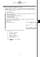
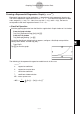
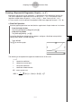
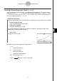
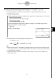
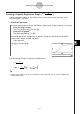
Table Of Contents
- Getting Ready
- Contents
- About This User’s Guide
- Chapter 1 Getting Acquainted
- Chapter 2 Using the Main Application
- 2-1 Main Application Overview
- 2-2 Basic Calculations
- 2-3 Using the Calculation History
- 2-4 Function Calculations
- 2-5 List Calculations
- 2-6 Matrix and Vector Calculations
- 2-7 Using the Action Menu
- 2-8 Using the Interactive Menu
- 2-9 Using the Main Application in Combination with Other Applications
- 2-10 Using Verify
- Chapter 3 Using the Graph & Table Application
- Chapter 4 Using the Conics Application
- Chapter 5 Using the 3D Graph Application
- Chapter 6 Using the Sequence Application
- Chapter 7 Using the Statistics Application
- 7-1 Statistics Application Overview
- 7-2 Using List Editor
- 7-3 Before Trying to Draw a Statistical Graph
- 7-4 Graphing Single-Variable Statistical Data
- 7-5 Graphing Paired-Variable Statistical Data
- 7-6 Using the Statistical Graph Window Toolbar
- 7-7 Performing Statistical Calculations
- 7-8 Test, Confidence Interval, and Distribution Calculations
- 7-9 Tests
- 7-10 Confidence Intervals
- 7-11 Distribution
- 7-12 Statistical System Variables
- Chapter 8 Using the Geometry Application
- Chapter 9 Using the Numeric Solver Application
- Chapter 10 Using the eActivity Application
- Chapter 11 Using the Presentation Application
- Chapter 12 Using the Program Application
- Chapter 13 Using the Spreadsheet Application
- Chapter 14 Using the Setup Menu
- Chapter 15 Configuring System Settings
- 15-1 System Setting Overview
- 15-2 Managing Memory Usage
- 15-3 Using the Reset Dialog Box
- 15-4 Initializing Your ClassPad
- 15-5 Adjusting Display Contrast
- 15-6 Configuring Power Properties
- 15-7 Specifying the Display Language
- 15-8 Specifying the Font Set
- 15-9 Specifying the Alphabetic Keyboard Arrangement
- 15-10 Optimizing “Flash ROM”
- 15-11 Specifying the Ending Screen Image
- 15-12 Adjusting Touch Panel Alignment
- 15-13 Viewing Version Information
- Chapter 16 Performing Data Communication
- Appendix
20050501
Drawing a Power Regression Graph (
y = a·x
b
)
Power regression can be used when y is proportional to the power of x. The normal power
regression formula is y = a · x
b
. If we obtain the logarithms of both sides, we get ln(y) = ln(a)
+ b · ln(x). Next, if we say that X = ln(x), Y = ln(y), and A = ln(a), the formula corresponds to
the linear regression formula Y = A + b·X.
u ClassPad Operation
Start the graphing operation from the Statistics application’s Graph window or List window.
From the Graph window
Tap [Calc] [Power Reg] [OK] [OK] ".
From the List window
Tap [SetGraph][Setting...], or G.
On the Set StatGraphs dialog box that appears, configure a StatGraph setup with the
setting shown below, and then tap [Set].
Type: PowerR
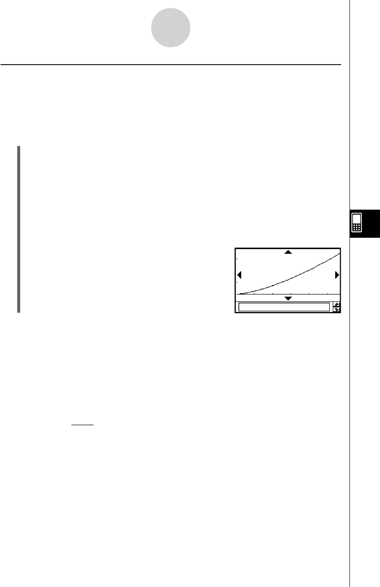
Tap y to draw the graph.
7-5-12
Graphing Paired-Variable Statistical Data
The following is the power regression model formula.
y = a·x
b
a : regression coefficient
b : regression power
r : correlation coefficient
r
2
: coefficient of determination
MSe :mean square error
• MSe =
Σ
1
n – 2
i=1
n
(ln (y
i
) – (ln (a) + b·ln (x
i
)))
2