
User Manual
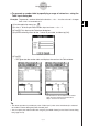
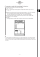
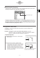
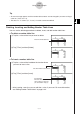
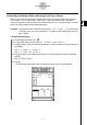
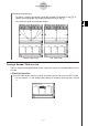
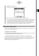
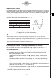
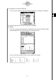
Table Of Contents
- Getting Ready
- Contents
- About This User’s Guide
- Chapter 1 Getting Acquainted
- Chapter 2 Using the Main Application
- 2-1 Main Application Overview
- 2-2 Basic Calculations
- 2-3 Using the Calculation History
- 2-4 Function Calculations
- 2-5 List Calculations
- 2-6 Matrix and Vector Calculations
- 2-7 Using the Action Menu
- 2-8 Using the Interactive Menu
- 2-9 Using the Main Application in Combination with Other Applications
- 2-10 Using Verify
- Chapter 3 Using the Graph & Table Application
- Chapter 4 Using the Conics Application
- Chapter 5 Using the 3D Graph Application
- Chapter 6 Using the Sequence Application
- Chapter 7 Using the Statistics Application
- 7-1 Statistics Application Overview
- 7-2 Using List Editor
- 7-3 Before Trying to Draw a Statistical Graph
- 7-4 Graphing Single-Variable Statistical Data
- 7-5 Graphing Paired-Variable Statistical Data
- 7-6 Using the Statistical Graph Window Toolbar
- 7-7 Performing Statistical Calculations
- 7-8 Test, Confidence Interval, and Distribution Calculations
- 7-9 Tests
- 7-10 Confidence Intervals
- 7-11 Distribution
- 7-12 Statistical System Variables
- Chapter 8 Using the Geometry Application
- Chapter 9 Using the Numeric Solver Application
- Chapter 10 Using the eActivity Application
- Chapter 11 Using the Presentation Application
- Chapter 12 Using the Program Application
- Chapter 13 Using the Spreadsheet Application
- Chapter 14 Using the Setup Menu
- Chapter 15 Configuring System Settings
- 15-1 System Setting Overview
- 15-2 Managing Memory Usage
- 15-3 Using the Reset Dialog Box
- 15-4 Initializing Your ClassPad
- 15-5 Adjusting Display Contrast
- 15-6 Configuring Power Properties
- 15-7 Specifying the Display Language
- 15-8 Specifying the Font Set
- 15-9 Specifying the Alphabetic Keyboard Arrangement
- 15-10 Optimizing “Flash ROM”
- 15-11 Specifying the Ending Screen Image
- 15-12 Adjusting Touch Panel Alignment
- 15-13 Viewing Version Information
- Chapter 16 Performing Data Communication
- Appendix
20050501
u Specifying all x-values
This method generates a reference table by looking up data stored in a list. A LIST variable is
used to specify the x-values. When using this method, it is up to you specify all of the correct
x-values required to generate the summary table. The summary table will not be generated
correctly if you provide incorrect x-values.
The following shows examples of each of the three available summary table generation
methods by generating a table for the function y = x
3
– 3x.
3-4-10
Using Table & Graph
x –1 0 1
f⬘(x)+ 0––3– 0+
f ⬙(x)– –6 – 0 + 6+
f (x) 2 0 –2
Tip
•You can control whether or not the summary table should include an f ⬙(x) line (quadratic
differential component) using the [Summary Table f ⬙(x)] setting on the [Cell] tab of the Basic
Format dialog box (page 14-3-3). Turning on the [Summary Table f ⬙(x)] option causes both linear
differential components and quadratic differential components to be displayed in the summary
table. Turning it off shows linear differential components only.
k Generating a Summary Table Using Automatically Set x-Values
With this method, the summary table is generated using a range of values from –∞ to ∞.
u ClassPad Operation
(1) On the Basic Format dialog box, select “View Window” for the [Summary Table] setting,
and specify the value you want for [Cell Width Pattern]. This example uses a [Cell
Width Pattern] setting of “4 Cells”.
•To open the Basic Format dialog box, tap O, [Settings], [Setup], and then [Basic
Format].
• For additional details about Basic Format settings, see “14-3 Setup Menu Settings”.
(2) Input the function y = x
3
– 3x on the Graph Editor window.
•Generation of summary tables is supported for “y=” type functions only.
•Clear the check boxes of all other functions on the Graph Editor window, if necessary.
Select the check box next to y = x
3
– 3x and press E.
• If the check boxes of more than one “y=” type functions are selected, the one with the
lowest line number (y1, y2, y3, etc.) is used for number table generation.
(3) Tap 6 to display the View Window dialog box.
Summary Table and Graph of y = x
3
– 3x
(The graph to the right is for reference only.)
2
1
–2
–1
–2
–1
1
2