
User Manual
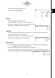

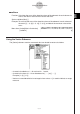
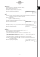
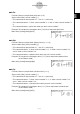
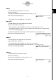
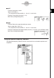
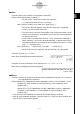
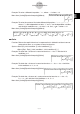
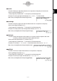
Table Of Contents
- Getting Ready
- Contents
- About This User’s Guide
- Chapter 1 Getting Acquainted
- Chapter 2 Using the Main Application
- 2-1 Main Application Overview
- 2-2 Basic Calculations
- 2-3 Using the Calculation History
- 2-4 Function Calculations
- 2-5 List Calculations
- 2-6 Matrix and Vector Calculations
- 2-7 Using the Action Menu
- 2-8 Using the Interactive Menu
- 2-9 Using the Main Application in Combination with Other Applications
- 2-10 Using Verify
- Chapter 3 Using the Graph & Table Application
- Chapter 4 Using the Conics Application
- Chapter 5 Using the 3D Graph Application
- Chapter 6 Using the Sequence Application
- Chapter 7 Using the Statistics Application
- 7-1 Statistics Application Overview
- 7-2 Using List Editor
- 7-3 Before Trying to Draw a Statistical Graph
- 7-4 Graphing Single-Variable Statistical Data
- 7-5 Graphing Paired-Variable Statistical Data
- 7-6 Using the Statistical Graph Window Toolbar
- 7-7 Performing Statistical Calculations
- 7-8 Test, Confidence Interval, and Distribution Calculations
- 7-9 Tests
- 7-10 Confidence Intervals
- 7-11 Distribution
- 7-12 Statistical System Variables
- Chapter 8 Using the Geometry Application
- Chapter 9 Using the Numeric Solver Application
- Chapter 10 Using the eActivity Application
- Chapter 11 Using the Presentation Application
- Chapter 12 Using the Program Application
- Chapter 13 Using the Spreadsheet Application
- Chapter 14 Using the Setup Menu
- Chapter 15 Configuring System Settings
- 15-1 System Setting Overview
- 15-2 Managing Memory Usage
- 15-3 Using the Reset Dialog Box
- 15-4 Initializing Your ClassPad
- 15-5 Adjusting Display Contrast
- 15-6 Configuring Power Properties
- 15-7 Specifying the Display Language
- 15-8 Specifying the Font Set
- 15-9 Specifying the Alphabetic Keyboard Arrangement
- 15-10 Optimizing “Flash ROM”
- 15-11 Specifying the Ending Screen Image
- 15-12 Adjusting Touch Panel Alignment
- 15-13 Viewing Version Information
- Chapter 16 Performing Data Communication
- Appendix
20050501
2-7-40
Using the Action Menu
Example: To solve a differential equation y’ = x, where y = 1 when x = 0.
Menu Item: [Action][Equation/Inequality][dSolve]
Example: To solve the system of first order differential equations y’ = y + z, z’ = y – z,
where “x” is the independent variable, “y” and “z” are the dependent variables,
and the initial conditions are y = 3 when x = 0, and z = 2 – 3 when x = 0
Menu Item: [Action][Equation/Inequality][dSolve]
uu
uu
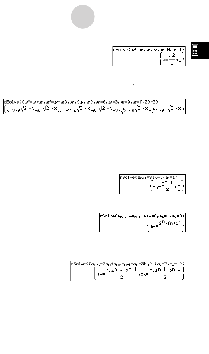
u rSolve
Function: Returns the explicit formula of a sequence that is defined in relation to one or
two previous terms, or a system of recursive formulas.
Syntax: rSolve (Eq, initial condition-1[, initial condition-2] [
)
]
rSolve ({Eq-1, Eq-2}, {initial condition-1, initial condition-2} [
)
]
Example: To obtain the n-th term of a recursion formula an+1 = 3an–1 with the initial
conditions a1=1
Menu Item: [Action][Equation/Inequality][rSolve]
Example: To obtain the n-th term of a recursion formula an+2 – 4an+1 + 4an = 0 with the
initial conditions a1 =1, a2 = 3
Menu Item: [Action][Equation/Inequality][rSolve]
Example: To obtain the n-th terms of a system of recursion formulas an+1 = 3an + bn,
bn+1 = an + 3bn with the initial conditions a1 =2, b1 = 1
Menu Item: [Action][Equation/Inequality][rSolve]