User Manual

20050501
2-7-39
Using the Action Menu
uu
uu
u solve
Function: Returns the solution of an equation or inequality.
Syntax: solve (Exp/Eq/Ineq [,variable] [ ) ]
• For this syntax, “Ineq” also includes the ≠ operator.
•“x” is the default when you omit “[,variable]”.
solve (Exp/Eq,variable[, value, lower limit, upper limit] [ ) ]
• This syntax does not support “Ineq”, but the ≠ operator is supported.
• “value” is an initially estimated value.
• This command is valid only for equations and ≠ expressions when “value”
and the items following it are included. In that case, this command returns
an approximate value.
•A true value is returned when you omit “value” and the items following it.
When, however, a true value cannot be obtained, an approximate value is
returned for equations only based on the assumption that value = 0, lower
limit = –⬁, and upper limit = ⬁.
solve ({Exp-1/Eq-1, ..., Exp-N/Eq-N}, {variable-1, ..., variable-N} [ ) ]
•When “Exp” is the first argument, the equation Exp = 0 is presumed.
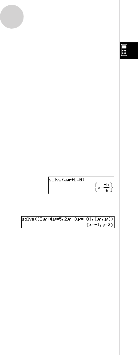
Example: To solve ax + b = 0 for x
Menu Item: [Action][Equation/Inequality][solve]
Example: To solve simultaneous linear equations 3x + 4y = 5, 2x – 3y = –8
Menu Item: [Action][Equation/Inequality][solve]
uu
uu
u dSolve
Function: Solves first, second or third order ordinary differential equations, or a system of
first order differential equations.
Syntax: dSolve (Eq, independent variable, dependent variable [, initial condition-1, initial
condition-2][, initial condition-3, initial condition-4][, initial condition-5, initial
condition-6] [ ) ]
dSolve ({Eq-1, Eq-2}, independent variable, {dependent variable-1, dependent
variable-2} [, initial condition-1, initial condition-2, initial condition-3, initial
condition-4] [ ) ]
• If you omit the initial conditions, the solution will include arbitrary constants.
• Input all initial conditions equations using the syntax Var = Exp. Any initial condition that
uses any other syntax will be ignored.