Chapter Statistical Graphs and Calculations This chapter describes how to input statistical data into lists, how to calculate the mean, maximum and other statistical values, how to perform various statistical tests, how to determine the confidence interval, and how to produce a distribution of statistical data. It also tells you how to perform regression calculations.
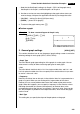
18-1 Before Performing Statistical Calculations In the Main Menu, select the STAT icon to enter the STAT Mode and display the statistical data lists. Use the statistical data lists to input data and to perform statistical calculations. Use f, c, d and e to move the highlighting around the lists. 250 P.251 • {GRPH} ... {graph menu} P.270 • {CALC} ... {statistical calculation menu} P.277 • {TEST} ... {test menu} P.294 • {INTR} ... {confidence interval menu} P.304 • {DIST} ...
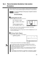
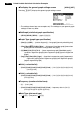
18-2 Paired-Variable Statistical Calculation Examples Once you input data, you can use it to produce a graph and check for tendencies. You can also use a variety of different regression calculations to analyze the data. Example To input the following two data groups and perform statistical calculations {0.5, 1.2, 2.4, 4.0, 5.2} {–2.1, 0.3, 1.5, 2.0, 2.4} k Inputting Data into Lists Input the two groups of data into List 1 and List 2. a.fwb.cw c.ewewf.cw e -c.bwa.dw b.fwcwc.
18 - 2 Paired-Variable Statistical Calculation Examples While the statistical data list is on the display, perform the following procedure. !Z2(Man) J(Returns to previous menu.) • It is often difficult to spot the relationship between two sets of data (such as height and shoe size) by simply looking at the numbers. Such relationship become clear, however, when we plot the data on a graph, using one set of values as x-data and the other set as y-data.
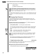
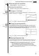
Paired-Variable Statistical Calculation Examples 18 - 2 • Note that the StatGraph1 setting is for Graph 1 (GPH1 of the graph menu), StatGraph2 is for Graph 2, and StatGraph3 is for Graph 3. 2. Use the cursor keys to move the highlighting to the graph whose status you want to change, and press the applicable function key to change the status. • {On}/{Off} ... setting {On (draw)}/{Off (non-draw)} • {DRAW} ... {draws all On graphs} 3. To return to the graph menu, press J.
18 - 2 Paired-Variable Statistical Calculation Examples uTo display the general graph settings screen [GRPH]-[SET] Pressing 6 (SET) displays the general graph settings screen. • The settings shown here are examples only. The settings on your general graph settings screen may differ. u StatGraph (statistical graph specification) • {GPH1}/{GPH2}/{GPH3} ... graph {1}/{2}/{3} u Graph Type (graph type specification) • {Scat}/{xy}/{NPP} ...
Paired-Variable Statistical Calculation Examples 18 - 2 uGraph Color (graph color specification) CFX • {Blue}/{Orng}/{Grn} ... {blue}/{orange}/{green} uOutliers (outliers specification) • {On}/{Off} ... {display}/{do not display} Med-Box outliers k Drawing an xy Line Graph P.254 (Graph Type) (xy) Paired data items can be used to plot a scatter diagram. A scatter diagram where the points are linked is an xy line graph. Press J or !Q to return to the statistical data list.
18 - 2 Paired-Variable Statistical Calculation Examples k Displaying Statistical Calculation Results Whenever you perform a regression calculation, the regression formula parameter (such as a and b in the linear regression y = ax + b) calculation results appear on the display. You can use these to obtain statistical calculation results. Regression parameters are calculated as soon as you press a function key to select a regression type while a graph is on the display.
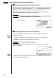
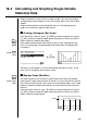
Calculating and Graphing Single-Variable Statistical Data 18-3 18 - 3 Calculating and Graphing Single-Variable Statistical Data Single-variable data is data with only a single variable. If you are calculating the average height of the members of a class for example, there is only one variable (height). Single-variable statistics include distribution and sum. The following types of graphs are available for single-variable statistics.
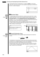
18 - 3 Calculating and Graphing Single-Variable Statistical Data To plot the data that falls outside the box, first specify “MedBox” as the graph type. Then, on the same screen you use to specify the graph type, turn the outliers item “On”, and draw the graph. k Mean-box Graph P.254 (Graph Type) (Box) This type of graph shows the distribution around the mean when there is a large number of data items.
Calculating and Graphing Single-Variable Statistical Data 18 - 3 k Broken Line Graph P.254 (Graph Type) (Brkn) A broken line graph is formed by plotting the data in one list against the frequency of each data item in another list and connecting the points with straight lines. Calling up the graph menu from the statistical data list, pressing 6 (SET), changing the settings to drawing of a broken line graph, and then drawing a graph creates a broken line graph.
18 - 3 Calculating and Graphing Single-Variable Statistical Data minX ............... minimum Q1 .................. first quartile Med ................ median Q3 .................. third quartile _ x –xσn ............ data mean – population standard deviation _ x + xσn ............ data mean + population standard deviation maxX .............. maximum Mod ................ mode • Press 6 (DRAW) to return to the original single-variable statistical graph.
18-4 Calculating and Graphing Paired-Variable Statistical Data Under “Plotting a Scatter Diagram,” we displayed a scatter diagram and then performed a logarithmic regression calculation. Let’s use the same procedure to look at the various regression functions. k Linear Regression Graph P.254 Linear regression plots a straight line that passes close to as many data points as possible, and returns values for the slope and y-intercept (y-coordinate when x = 0) of the line.
18 - 4 Calculating and Graphing Paired-Variable Statistical Data 6(DRAW) a ...... Med-Med graph slope b ...... Med-Med graph y-intercept k Quadratic/Cubic/Quartic Regression Graph P.254 A quadratic/cubic/quartic regression graph represents connection of the data points of a scatter diagram. It actually is a scattering of so many points that are close enough together to be connected. The formula that represents this is quadratic/cubic/quartic regression. Ex.
Calculating and Graphing Paired-Variable Statistical Data 18 - 4 k Logarithmic Regression Graph P.254 Logarithmic regression expresses y as a logarithmic function of x. The standard logarithmic regression formula is y = a + b × Inx, so if we say that X = Inx, the formula corresponds to linear regression formula y = a + bX. 6(g)1(Log) 1 2 3 4 5 6 6(DRAW) a ...... regression constant term b ...... regression coefficient r ...... correlation coefficient r2 .....
18 - 4 Calculating and Graphing Paired-Variable Statistical Data k Power Regression Graph P.254 Exponential regression expresses y as a proportion of the power of x. The standard power regression formula is y = a × xb, so if we take the logarithm of both sides we get Iny = Ina + b × Inx. Next, if we say X = Inx, Y = Iny, and A = Ina, the formula corresponds to linear regression formula Y = A + bX. 6(g)3(Pwr) 1 2 3 4 5 6 6(DRAW) a ...... regression coefficient b ...... regression power r ......
Calculating and Graphing Paired-Variable Statistical Data 18 - 4 Gas bills, for example, tend to be higher during the winter when heater use is more frequent. Periodic data, such as gas usage, is suitable for application of sine regression.
- 4 Calculating and Graphing Paired-Variable Statistical Data C 1 + ae–bx y= 6(g)6(g)1(Lgst) 6 6(DRAW) Example Imagine a country that started out with a television diffusion rate of 0.3% in 1966, which grew rapidly until diffusion reached virtual saturation in 1980. Use the paired statistical data shown below, which tracks the annual change in the diffusion rate, to perform logistic regression.
Calculating and Graphing Paired-Variable Statistical Data 18 - 4 Draw a logistic regression graph based on the parameters obtained from the analytical results. 6(DRAW) k Residual Calculation Actual plot points (y-coordinates) and regression model distance can be calculated during regression calculations. P.6 While the statistical data list is on the display, recall the set up screen to specify a list (“List 1” through “List 6”) for “Resid List”. Calculated residual data is stored in the specified list.
18 - 4 Calculating and Graphing Paired-Variable Statistical Data • Use c to scroll the list so you can view the items that run off the bottom of the screen. _ x ..................... mean of xList data Σ x ................... sum of xList data Σ x2 .................. sum of squares of xList data xσn .................. population standard deviation of xList data xσn-1 ................ sample standard deviation of xList data n ..................... number of xList data items _ y .....................
Calculating and Graphing Paired-Variable Statistical Data 18 - 4 k Multiple Graphs P.252 You can draw more than one graph on the same display by using the procedure under “Changing Graph Parameters” to set the graph draw (On)/non-draw (Off) status of two or all three of the graphs to draw “On”, and then pressing 6 (DRAW). After drawing the graphs, you can select which graph formula to use when performing single-variable statistic or regression calculations. 6(DRAW) P.
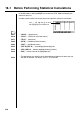
18 - 5 18-5 Performing Statistical Calculations Performing Statistical Calculations All of the statistical calculations up to this point were performed after displaying a graph. The following procedures can be used to perform statistical calculations alone. uTo specify statistical calculation data lists You have to input the statistical data for the calculation you want to perform and specify where it is located before you start a calculation. Display the statistical data and then press 2(CALC)6 (SET).
Performing Statistical Calculations 18 - 5 Now you can use the cursor keys to view the characteristics of the variables. P.259 For details on the meanings of these statistical values, see “Displaying SingleVariable Statistical Results”. k Paired-Variable Statistical Calculations In the previous examples from “Linear Regression Graph” to “Logistic Regression Graph,” statistical calculation results were displayed after the graph was drawn.
18 - 5 Performing Statistical Calculations k Estimated Value Calculation ( , ) After drawing a regression graph with the STAT Mode, you can use the RUN Mode to calculate estimated values for the regression graph's x and y parameters. • Note that you cannot obtain estimated values for a Med-Med, quadratic regression, cubic regression, quartic regression, sine regression, or logistic regression graph.
Performing Statistical Calculations 18 - 5 k Normal Probability Distribution Calculation and Graphing You can calculate and graph normal probability distributions for single-variable statistics. uNormal probability distribution calculations Use the RUN Mode to perform normal probability distribution calculations. Press K in the RUN Mode to display the option number and then press 6 (g) 3 (PROB) 6 (g) to display a function menu, which contains the following items. • {P(}/{Q(}/{R(} ...
18 - 5 Performing Statistical Calculations 2. Use the STAT Mode to perform the single-variable statistical calculations. 2(CALC)6(SET) 1(List1)c3(List2)J1(1VAR) 3. Press m to display the Main Menu, and then enter the RUN Mode. Next, press K to display the option menu and then 6 (g) 3 (PROB) 6 (g). • You obtain the normalized variate immediately after performing singlevariable statistical calculations only. 4(t () bga.f)w (Normalized variate t for 160.5cm) Result: –1.633855948 ( –1.634) 4(t() bhf.
Performing Statistical Calculations 18 - 5 k Normal Probability Graphing You can graph a normal probability distribution with Graph Y = in the Sketch Mode. Example To graph normal probability P(0.5) Perform the following operation in the RUN Mode. !4(Sketch)1(Cls)w 5(GRPH)1(Y=)K6(g)3(PROB) 6(g)1(P()a.f)w The following shows the View Window settings for the graph. Ymin ~ Ymax –0.1 0.45 Xmin ~ Xmax –3.2 3.
18-6 Tests The Z Test provides a variety of different standardization-based tests. They make it possible to test whether or not a sample accurately represents the population when the standard deviation of a population (such as the entire population of a country) is known from previous tests. Z testing is used for market research and public opinion research, that need to be performed repeatedly. 1-Sample Z Test tests for unknown population mean when the population standard deviation is known.
Tests 18 - 6 2-Sample F Test tests the hypothesis that there will be no change in the result for a population when a result of a sample is composed of multiple factors and one or more of the factors is removed. It could be used, for example, to test the carcinogenic effects of multiple suspected factors such as tobacco use, alcohol, vitamin deficiency, high coffee intake, inactivity, poor living habits, etc.
18 - 6 Tests The following shows the meaning of each item in the case of list data specification. Data ................ data type µ ..................... population mean value test conditions (“G µ0” specifies two-tail test, “< µ0” specifies lower one-tail test, “> µ0” specifies upper one-tail test.) µ0 .................... assumed population mean σ ..................... population standard deviation (σ > 0) List .................. list whose contents you want to use as data (List 1 to 6) Freq ...........
Tests 18 - 6 Perform the following key operations from the statistical result screen. J(To data input screen) cccccc(To Execute line) 6(DRAW) u 2-Sample Z Test This test is used when the sample standard deviations for two populations are known to test the hypothesis. The 2-Sample Z Test is applied to the normal distribution.
18 - 6 Tests The following shows the meaning of parameter data specification items that are different from list data specification. o1 .................... n1 .................... o2 .................... n2 .................... Example sample 1 mean sample 1 size (positive integer) sample 2 mean sample 2 size (positive integer) To perform a 2-Sample Z Test when two lists of data are input For this example, we will perform a µ1 < µ2 test for the data List1 = {11.2, 10.9, 12.5, 11.3, 11.7} and List2 = {0.
Tests 18 - 6 u 1-Prop Z Test This test is used to test for an unknown proportion of successes. The 1-Prop Z Test is applied to the normal distribution. x – p0 n Z= p0 (1– p0) n p0 : expected sample proportion n : sample size Perform the following key operations from the statistical data list. 3(TEST) 1(Z) 3(1-P) Prop ................ sample proportion test conditions (“G p0” specifies two-tail test, “< p0” specifies lower one-tail test, “> p0” specifies upper one-tail test.) p0 ....................
18 - 6 Tests The following key operations can be used to draw a graph. J cccc 6(DRAW) u 2-Prop Z Test This test is used to compare the proportion of successes. The 2-Prop Z Test is applied to the normal distribution. x1 x2 n1 – n2 Z= p(1 – p ) 1 + 1 n1 n2 x1 : sample 1 data value x2 : sample 2 data value n1 : sample 1 size n2 : sample 2 size p̂ : estimated sample proportion Perform the following key operations from the statistical data list. 3(TEST) 1(Z) 4(2-P) p1 ....................
Tests 18 - 6 3(>)c ccfw daaw cdaw daaw 1(CALC) p1>p2 ............... z ...................... p ..................... p̂1 .................... p̂2 .................... p̂ ..................... n1 .................... n2 .................... direction of test z value p-value estimated proportion of population 1 estimated proportion of population 2 estimated sample proportion sample 1 size sample 2 size The following key operations can be used to draw a graph.
18 - 6 Tests The following shows the meaning of each item in the case of list data specification. Data ................ data type µ ..................... population mean value test conditions (“G µ0” specifies twotail test, “< µ0” specifies lower one-tail test, “> µ0” specifies upper one-tail test.) µ0 .................... assumed population mean List .................. list whose contents you want to use as data Freq ................ frequency Execute ..........
Tests 18 - 6 u 2-Sample t Test 2-Sample t Test compares the population means when the population standard deviations are unknown. The 2-Sample t Test is applied to t-distribution. The following applies when pooling is in effect.
18 - 6 Tests The following shows the meaning of each item in the case of list data specification. Data ................ data type µ1 .................... sample mean value test conditions (“G µ2” specifies two-tail test, “< µ2” specifies one-tail test where sample 1 is smaller than sample 2, “> µ2” specifies one-tail test where sample 1 is greater than sample 2.) List1 ................ list whose contents you want to use as sample 1 data List2 ................
Tests 18 - 6 µ1Gµ2 .............. direction of test t ...................... p ..................... df .................... o1 .................... o2 .................... x1σn-1 ............... x2σn-1 ............... n1 .................... n2 .................... t value p-value degrees of freedom sample 1 mean sample 2 mean sample 1 standard deviation sample 2 standard deviation sample 1 size sample 2 size Perform the following key operations to display a graph.
18 - 6 Tests The following shows the meaning of each item in the case of list data specification. β & ρ ............... p-value test conditions (“G 0” specifies two-tail test, “< 0” specifies lower one-tail test, “> 0” specifies upper one-tail test.) XList ............... list for x-axis data YList ............... list for y-axis data Freq ................ frequency Execute ..........
Tests 18 - 6 k Other Tests u χ2 Test χ2 Test sets up a number of independent groups and tests hypotheses related to the proportion of the sample included in each group. The χ2 Test is applied to dichotomous variables (variable with two possible values, such as yes/no). k expected counts Σ x ×Σ x ij Fij = i=1 ij j=1 k ΣΣ x ij i=1 j=1 (xij – Fij)2 Fij i =1 j =1 k χ2 = Σ Σ For the above, data must already be input in a matrix using the MAT Mode.
18 - 6 Tests χ2 .................... χ2 value p ..................... p-value df .................... degrees of freedom Expected ........ expected counts (Result is always stored in MatAns.) The following key operations can be used to display the graph. J c 6(DRAW) u 2-Sample F Test 2-Sample F Test tests the hypothesis that when a sample result is composed of multiple factors, the population result will be unchanged when one or some of the factors are removed.
Tests 18 - 6 The following shows the meaning of parameter data specification items that are different from list data specification. x1σn-1 ............... n1 .................... x2σn-1 ............... n2 ....................
18 - 6 Tests u Analysis of Variance (ANOVA) ANOVA tests the hypothesis that when there are multiple samples, the means of the populations of the samples are all equal.
Tests 18 - 6 2(3)c 1(List1)c 2(List2)c 3(List3)c 1(CALC) F ..................... p ..................... xpσn-1 ............... Fdf .................. SS ................... MS .................. Edf .................. SSe ................. MSe ................
18 - 8 18-7 Confidence Interval Confidence Interval A confidence interval is a range (interval) that includes a statistical value, usually the population mean. A confidence interval that is too broad makes it difficult to get an idea of where the population value (true value) is located. A narrow confidence interval, on the other hand, limits the population value and makes it difficult to obtain reliable results. The most commonly used confidence levels are 95% and 99%.
Confidence Interval 18 - 7 k Z Confidence Interval You can use the following menu to select from the different types of Z confidence interval. • {1-S}/{2-S}/{1-P}/{2-P} ... {1-Sample}/{2-Sample}/{1-Prop}/{2-Prop} Z Interval u 1-Sample Z Interval 1-Sample Z Interval calculates the confidence interval for an unknown population mean when the population standard deviation is known. The following is the confidence interval. Left = o – Z α σ 2 n Right = o + Z α σ 2 n However, α is the level of significance.
18 - 7 Confidence Interval Example To calculate the 1-Sample Z Interval for one list of data For this example, we will obtain the Z Interval for the data {11.2, 10.9, 12.5, 11.3, 11.7}, when C-Level = 0.95 (95% confidence level) and σ = 3. 1(List)c a.jfw dw 1(List1)c1(1)c1(CALC) Left ................. interval lower limit (left edge) Right ............... interval upper limit (right edge) o ..................... sample mean xσn-1 ................ sample standard deviation n .....................
Confidence Interval 18 - 7 σ1 .................... population standard deviation of sample 1 (σ1 > 0) σ2 .................... population standard deviation of sample 2 (σ2 > 0) List1 ................ list whose contents you want to use as sample 1 data List2 ................ list whose contents you want to use as sample 2 data Freq1 .............. frequency of sample 1 Freq2 .............. frequency of sample 2 Execute ..........
18 - 7 Confidence Interval u 1-Prop Z Interval 1-Prop Z Interval uses the number of data to calculate the confidence interval for an unknown proportion of successes. The following is the confidence interval. The value 100 (1 – α) % is the confidence level. x Left = n – Z α 2 x Right = n + Z α 2 1 x x n n 1– n n : sample size x : data 1 x x n n 1– n Perform the following key operations from the statistical data list. 4(INTR) 1(Z) 3(1-P) Data is specified using parameter specification.
Confidence Interval 18 - 7 u 2-Prop Z Interval 2-Prop Z Interval uses the number of data items to calculate the confidence interval for the defference between the proportion of successes in two populations. The following is the confidence interval. The value 100 (1 – α) % is the confidence level.
18 - 7 Confidence Interval p̂1 .................... p̂2 .................... n1 .................... n2 .................... estimated sample propotion for sample 1 estimated sample propotion for sample 2 sample 1 size sample 2 size k t Confidence Interval You can use the following menu to select from two types of t confidence interval. • {1-S}/{2-S} ...
Confidence Interval Example 18 - 7 To calculate the 1-Sample t Interval for one list of data For this example, we will obtain the 1-Sample t Interval for data = {11.2, 10.9, 12.5, 11.3, 11.7} when C-Level = 0.95. 1(List)c a.jfw 1(List1)c 1(1)c 1(CALC) Left ................. interval lower limit (left edge) Right ............... interval upper limit (right edge) o ..................... sample mean xσn-1 ................ sample standard deviation n .....................
18 - 7 Confidence Interval Perform the following key operations from the statistical data list. 4(INTR) 2(t) 2(2-S) The following shows the meaning of each item in the case of list data specification. Data ................ data type C-Level ........... confidence level (0 < C-Level < 1) List1 ................ list whose contents you want to use as sample 1 data List2 ................ list whose contents you want to use as sample 2 data Freq1 .............. frequency of sample 1 Freq2 ..............
Confidence Interval Example 18 - 7 To calculate the 2-Sample t Interval when two lists of data are input For this example, we will obtain the 2-Sample t Interval for data 1 = {55, 54, 51, 55, 53, 53, 54, 53} and data 2 = {55.5, 52.3, 51.8, 57.2, 56.5} without pooling when C-Level = 0.95. 1(List)c a.jfw 1(List1)c2(List2)c1(1)c 1(1)c2(Off)c1(CALC) Left ................. interval lower limit (left edge) Right ............... interval upper limit (right edge) df .................... o1 ....................
18-8 Distribution There is a variety of different types of distribution, but the most well-known is “normal distribution,” which is essential for performing statistical calculations. Normal distribution is a symmetrical distribution centered on the greatest occurrences of mean data (highest frequency), with the frequency decreasing as you move away from the center. Poisson distribution, geometric distribution, and various other distribution shapes are also used, depending on the data type.
Distribution 18 - 8 k Normal Distribution You can use the following menu to select from the different types of calculation. • {Npd}/{Ncd}/{InvN} ... {normal probability density}/{normal distribution probability}/{inverse cumulative normal distribution} calculation u Normal probability density Normal probability density calculates the probability density of normal distribution from a specified x value. Normal probability density is applied to the standard normal distribution.
18 - 8 Distribution Perform the following key operations to display a graph. J ccc 6(DRAW) uNormal distribution probability Normal distribution probability calculates the probability of normal distribution data falling between two specific values. p= 1 2πσ ∫ 2 b e a – (x – µ µ) 2σ 2 dx a : lower boundary b : upper boundary Perform the following key operations from the statistical data list. 5(DIST) 1(NORM) 2(Ncd) Data is specified using parameter specification.
Distribution 18 - 8 • This calculator performs the above calculation using the following: ∞ = 1E99, –∞ = –1E99 u Inverse cumulative normal distribution Inverse cumulative normal distribution calculates a value that represents the location within a normal distribution for a specific cumulative probability. ∫ −∞ f (x)dx = p Upper boundary of integration interval α=? Specify the probability and use this formula to obtain the integration interval.
18 - 8 Distribution k Student-t Distribution You can use the following menu to select from the different types of Student-t distribution. • {tpd}/{tcd} ... {Student-t probability density}/{Student-t distribution probability} calculation uStudent-t probability density Student-t probability density calculates t probability density from a specified x value. df + 1 1 + x2 df 2 f (x) = π df df Γ 2 Γ – df+1 2 Perform the following key operations from the statistical data list.
Distribution 18 - 8 Perform the following key operation to display a graph. J cc 6(DRAW) u Student-t distribution probability Student-t distribution probability calculates the probability of t distribution data falling between two specific values. df + 1 2 p= df Γ 2 π df Γ ∫ b a 1 + x2 df – df+1 2 dx a : lower boundary b : upper boundary Perform the following key operations from the statistical data list. 5(DIST) 2(t) 2(tcd) Data is specified using parameter specification.
18 - 8 Distribution k Chi-square Distribution You can use the following menu to select from the different types of chi-square distribution. • {Cpd}/{Ccd} ... {χ2 probability density}/{χ2 distribution probability} calculation uχ2 probability density χ2 probability density calculates the probability density function for the χ2 distribution at a specified x value. f (x) = 1 df Γ 2 1 2 df 2 df –1 – x2 e x 2 (x > 0) Perform the following key operations from the statistical data list.
Distribution 18 - 8 Perform the following key operations to display a graph. J cc 6(DRAW) uχ2 distribution probability χ2 distribution probability calculates the probability of χ2 distribution data falling between two specific values. p= 1 df Γ 2 1 2 df 2 ∫ b x df x –1 – 2 2 e dx a : lower boundary b : upper boundary a Perform the following key operations from the statistical data list. 5(DIST) 3(CHI) 2(Ccd) Data is specified using parameter specification.
18 - 8 Distribution k F Distribution You can use the following menu to select from the different types of F distribution. • {Fpd}/{Fcd} ... {F probability density}/{F distribution probability} calculation u F probability density F probability density calculates the probability density function for the F distribution at a specified x value. n+d 2 f (x) = n d Γ Γ 2 2 Γ n d n 2 x n –1 2 1 + nx d – n+d 2 (x > 0) Perform the following key operations from the statistical data list.
Distribution 18 - 8 u F distribution probability F distribution probability calculates the probability of F distribution data falling between two specific values. n+d 2 p= n d Γ Γ 2 2 Γ n d n 2 ∫ b x n –1 2 a 1 + nx d – a : lower boundary b : upper boundary n+d 2 dx Perform the following key operations from the statistical data list. 5(DIST) 4(F) 2(Fcd) Data is specified using parameter specification. The following shows the meaning of each item. Lower ............. lower boundary Upper ...
18 - 8 Distribution uBinomial probability Binomial probability calculates a probability at specified value for the discrete binomial distribution with the specified number of trials and probability of success on each trial. f (x) = n C x px (1–p) n – x (x = 0, 1, ·······, n) p : success probability (0 < p < 1) n : number of trials Perform the following key operations from the statistical data list.
Distribution 18 - 8 uBinomial cumulative density Binomial cumulative density calculates a cumulative probability at specified value for the discrete binomial distribution with the specified number of trials and probability of success on each trial. Perform the following key operations from the statistical data list. 5(DIST) 5(BINM) 2(Bcd) The following shows the meaning of each item when data is specified using list specification. Data ................ data type List ..................
18 - 8 Distribution k Poisson Distribution You can use the following menu to select from the different types of Poisson distribution. • {Ppd}/{Pcd} ... {Poisson probability}/{Poisson cumulative density} calculation uPoisson probability Poisson probability calculates a probability at specified value for the discrete Poisson distribution with the specified mean. f (x) = e– µ µ x x! (x = 0, 1, 2, ···) µ : mean (µ > 0) Perform the following key operations from the statistical data list.
Distribution 18 - 8 u Poisson cumulative density Poisson cumulative density calculates a cumulative probability at specified value for the discrete Poisson distribution with the specified mean. Perform the following key operations from the statistical data list. 5(DIST) 6(g) 1(POISN) 2(Pcd) The following shows the meaning of each item when data is specified using list specification. Data ................ data type List .................. list whose contents you want to use as sample data µ .............
18 - 8 Distribution uGeometric probability Geometric probability calculates a probability at specified value, the number of the trial on which the first success occurs, for the discrete geometric distribution with the specified probability of success. f (x) = p(1– p) x – 1 (x = 1, 2, 3, ···) Perform the following key operations from the statistical data list. 5(DIST) 6(g) 2(GEO) 1(Gpd) The following shows the meaning of each item when data is specified using list specification. Data ................
Distribution 18 - 8 uGeometric cumulative density Geometric cumulative density calculates a cumulative probability at specified value, the number of the trial on which the first success occurs, for the discrete geometric distribution with the specified probability of success. Perform the following key operations from the statistical data list. 5(DIST) 6(g) 2(GEO) 2(Gcd) The following shows the meaning of each item when data is specified using list specification. Data ................ data type List .....
98