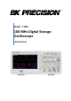
Model: 2190E 100 MHz Digital Storage Oscilloscope USER MANUAL
Safety Summary The following safety precautions apply to both operating and maintenance personnel and must be followed during all phases of operation, service, and repair of this instrument. Before applying power to this instrument: Read and understand the safety and operational information in this manual. Apply all the listed safety precautions. Verify that the voltage selector at the line power cord input is set to the correct line voltage.
battery. Category II (CAT II): Measurement instruments whose measurement inputs are meant to be connected to the mains supply at a standard wall outlet or similar sources. Example measurement environments are portable tools and household appliances. Category III (CAT III): Measurement instruments whose measurement inputs are meant to be connected to the mains installation of a building. Examples are measurements inside a building's circuit breaker panel or the wiring of permanently-installed motors.
To minimize shock hazard, the instrument chassis and cabinet must be connected to an electrical safety ground. This instrument is grounded through the ground conductor of the supplied, three-conductor AC line power cable. The power cable must be plugged into an approved threeconductor electrical outlet. The power jack and mating plug of the power cable meet IEC safety standards. Do not alter or defeat the ground connection.
The instrument is designed to be used in office-type indoor environments. Do not operate the instrument In the presence of noxious, corrosive, or flammable fumes, gases, vapors, chemicals, or finely-divided particulates. In relative humidity conditions outside the instrument's specifications. In environments where there is a danger of any liquid being spilled on the instrument or where any liquid can condense on the instrument. In air temperatures exceeding the specified operating temperatures.
Notify B&K Precision of the nature of any contamination of the instrument. Clean the instrument only as instructed Do not clean the instrument, its switches, or its terminals with contact cleaners, abrasives, lubricants, solvents, acids/bases, or other such chemicals. Clean the instrument only with a clean dry lint-free cloth or as instructed in this manual.
for both DC and AC voltages. Do not attempt any service or adjustment unless another person capable of rendering first aid and resuscitation is present. Do not insert any object into an instrument's ventilation openings or other openings. Hazardous voltages may be present in unexpected locations in circuitry being tested when a fault condition in the circuit exists. Servicing Do not substitute parts that are not approved by B&K Precision or modify this instrument.
For continued safe use of the instrument Do not place heavy objects on the instrument. Do not obstruct cooling air flow to the instrument. Do not place a hot soldering iron on the instrument. Do not pull the instrument with the power cord, connected probe, or connected test lead. Do not move the instrument when a probe is connected to a circuit being tested.
Compliance Statements Disposal of Old Electrical & Electronic Equipment (Applicable in the European Union and other European countries with separate collection systems) This product is subject to Directive 2002/96/EC of the European Parliament and the Council of the European Union on waste electrical and electronic equipment (WEEE), and in jurisdictions adopting that Directive, is marked as being put on the market after August 13, 2005, and should not be disposed of as unsorted municipal waste.
CE Declaration of Conformity This instrument meets the requirements of 2006/95/EC Low Voltage Directive and 2004/108/EC Electromagnetic Compatibility Directive with the following standards.
Safety Symbols Refer to the user manual for warning information to avoid hazard or personal injury and prevent damage to instrument. Electric Shock hazard Alternating current (AC) Chassis (earth ground) symbol. Ground terminal On (Power). This is the In position of the power switch when instrument is ON. Off (Power). This is the Out position of the power switch when instrument is OFF. Off (Supply). This is the AC mains connect/disconnect switch on top of the instrument.
Table of Contents Safety Summary ........................................................................................i Compliance Statements ........................................................................ viii Safety Symbols ......................................................................................... x 1 General Information .........................................................................1 1.1 Product Overview ...............................................................
3.4 Default Setup .............................................................................. 19 3.5 Universal Knob............................................................................ 23 3.6 Vertical System ........................................................................... 23 Using Vertical Position Knob and Volts/div Knob ............................... 24 3.7 Channel Function Menu ............................................................. 25 Setting up Channels .....................
Pass/Fail............................................................................................ 120 Waveform Record ............................................................................ 125 Recorder (Scan Mode Only) ............................................................. 129 Help Menu ........................................................................................ 134 Education Mode ...............................................................................
1 General Information 1.1 Product Overview The B&K Precision 2190E digital storage oscilloscope (DSO) is a portable benchtop instrument used for making measurements of signals and waveforms. The oscilloscope’s bandwidth is capable of capturing up to 100 MHz signals with a real time sampling rate of up to 1 GSa/s. With up to 40k points of deep memory, more details of a signal can be captured and displayed on a large color LCD display for analysis.
Certificate of calibration Verify that all items above are included in the shipping container. If anything is missing, please contact B&K Precision. 1.3 Front Panel It is important for you to familiarize yourself with the DSO’s front panel before operating the instrument. Below is a brief introduction of the front panel function operation. 10 9 8 7 6 5 1 2 Figure 1.
4 Probe Compensator (1 kHz and Ground) 5 Horizontal Controls (Time Base) 6 Trigger Controls 7 Auto Setup Button 8 Menu and Measurement Buttons 9 Universal Knob 10 Vertical Controls 1.4 Back Panel The following images show back and side panel connection locations. 6 5 1 2 3 Figure 1.
Back Panel Description 1 Security Lock Receptacle 2 LAN Interface 3 Pass/Fail Output 4 Rear USB (Type B) Device Connector 5 Power Input Connector 6 AC Power Switch 1.5 Display Information Figure 1.
User Interface Description 1 Trigger Status 2 USB Host Port Connection Indicator 3 Waveform Display Preview 4 Horizontal Trigger Position Marker 5 LAN Port Connection Indicator 6 Menu 7 Trigger Source, Type, and Level Indicator 8 Frequency Counter 9 Horizontal Delay Position 10 Horizontal Time Base Setting 11 Channel Source, Coupling Type, Volts/Division, BW Limit Indicator 12 Vertical Display Markers (Ground Reference) 13 Trigger Level Display Marker 5
2 Getting Started Before connecting and powering up the instrument, please review and go through the instructions in this chapter. 2.
Verify AC Input Voltage Verify and check to make sure proper AC voltages are available to power the instrument. The AC voltage range must meet the acceptable specification as explained in section 2.1. Connect Power Connect AC power cord to the AC receptacle in the rear panel and press the power switch to the ON position to turn ON the instrument. The instrument will have a boot screen while loading, after which the main screen will be displayed.
Check Model and Firmware Version The model and firmware version can be verified from within the menu system. Press Utility and select System Status option. The software/firmware version, hardware version, model, and serial number will be displayed. Press the Single key to exit. Function Check Follow the steps below to do a quick check of the oscilloscope’s functionality. 1. Power on the oscilloscope. Press “DEFAULT SETUP” to show the result of the self-check. The probe default attenuation is 1X.
PROBE COMP CH1 Figure 2.3 – Probe Compensation 3. Press “AUTO” to show the 1 kHz frequency and about 3V peakpeak square wave in couple seconds. Figure 2.4 – 3 Vpp Square Wave 4. Press “CH1” two times to turn off channel 1, Press“CH2” to change screen into channel 2, reset the channel 2 as step 2 and step 3.
Probe Safety A guard around the probe body provides a finger barrier for protection from electric shock. Figure 2.5 – Oscilloscope Probe Connect the probe to the oscilloscope and connect the ground terminal to ground before you take any measurements. SHOCK HAZARD To avoid electric shock when using the probe, keep fingers behind the guard on the probe body. To avoid electric shock while using the probe, do not touch metallic portions of the probe head while it is connected to a voltage source.
Probe Attenuation Probes are available with various attenuation factors which affect the vertical scale of the signal. The Probe Check function verifies that the Probe attenuation option matches the attenuation of the probe. You can push a vertical menu button (such as the CH 1 MENU button), and select the Probe option that matches the attenuation factor of your probe. NOTE: The default setting for the Probe option is 1X.
AUTO BUTTON PROBE COMP CH1 Figure 2.6 – Probe Compensation Setup 1. 2. 3. Set the Probe option attenuation in the channel menu to 10X. Do so by pressing CH1 button and selecting “Probe” from menu. Select 10X. Set the switch to 10X on the probe and connect the probe to channel 1 on the oscilloscope. If you use the probe hook-tip, ensure a proper connection by firmly inserting the tip onto the probe.
3 Functions and Operating Descriptions To use your oscilloscope effectively, you need to learn about the following oscilloscope functions: • • • • • • • • • • • • • • • • • Menu and control button Connector Auto Setup Default Setup Universal knob Vertical System Channel Function Menu Math Functions Using REF Horizontal System Trigger System Acquiring signals System Display System Measuring waveforms System Utility System Storage System Online Help function 13
3.1 Menu and Control Button Figure 3.1 – Control Buttons Channel buttons (CH1, CH2): Press a channel button to turn that channel ON or OFF and open the channel menu for that channel. You can use the channel menu to set up a channel. When the channel is on, the channel button is lit. MATH: Press to display the Math menu. You can use the MATH menu to use the oscilloscope’s Math functions. REF: Press to display the Ref Wave menu.
HORI MENU: Press to display the Horizontal menu. You can use the Horizontal menu to display the waveform and zoom in a segment of a waveform. TRIG MENU: Press to display the Trigger menu. You can use the Trigger menu to set the trigger type (Edge. Pulse, Video, Slope, Alternative) and trigger settings. SET TO 50%: Press to stabilize a waveform quickly. The oscilloscope can set the trigger level to be halfway between the minimum and maximum voltage level automatically.
sound, language, counter, etc. You can also view system status and update software. DEFAULT SETUP: Press to reset the oscilloscope’s settings to the default factory configuration. HELP: Enter the online help system. AUTO: Automatically sets the oscilloscope controls to produce a usable display of the input signals. RUN/STOP: Continuously acquires waveforms or stops the acquisition.
3.3 Auto Setup The 2190E Digital Storage Oscilloscope has an Auto Setup function that identifies the waveform types and automatically adjusts controls to produce a usable display of the input signal. Press the AUTO front panel button, and then press the menu option button adjacent to the desired waveform as follows: Figure 3.3 – Auto Setup Table 3.1 – Autoset Menu Option (Multi-cycle sine) (Single-cycle sine) Description Auto set the screen and display several cycles signal.
Auto set and show the rising time. (Rising edge) Auto set and show the falling time. (Falling edge) (Undo Setup) Causes the oscilloscope to recall the previous setup. Auto Set determines the trigger source based on the following conditions: • If multiple channels have signals, channel with the lowest frequency signal. • No signals found, the lowest-numbered channel displayed when Auto set was invoked. • No signals found and no channels displayed, oscilloscope displays and uses channel 1. Table 3.
V/div Adjusted VOLTS/DIV adjustability Coarse Signal inverted Off Horizontal position Center Time/div Adjusted Trigger type Edge Trigger source Auto detect the channel which has the input signal Trigger slope Rising Trigger mode Auto Trigger coupling DC Trigger holdoff Minimum Trigger level Set to 50% NOTE: The AUTO button can be disabled. Please see “Education Mode” for details. 3.4 Default Setup The oscilloscope is set up for normal operation when it is shipped from the factory.
• • • • • Language option Saved reference waveform files Saved setup files Display contrast Calibration data Table 3.3 – Default Setup Table Menu or system CH1,CH2 Options, knobs or buttons Default setup Coupling DC BW limit Off Volts/div Coarse Probe 1X Invert Off Filter Off Volts/div 1.00V Operation CH1+CH2 CH1 Invert Off CH2 Invert Off FFT operation: MATH HORIZONTAL CURSOR Source Window FFT Zoom Scale CH1 Hanning 1X dBVrms Display Split Window Main Position 0.
Source CH1 Horizontal (voltage) +/-3.2divs Vertical (time) +/-5divs three mode options Sampling Averages 16 Sampling mode Real Time Type Vectors Persist off ACQUIRE Gird DISPLAY SAVE/RECALL REF UTILITY TRIGGER (edge) Intensity 60% Brightness 40% Format YT Menu Display infinite Type Setups Save To Device Setup No.
TRIGGER (pulse) TRIGGER (Video) TRIGGER (Slope) TRIGGER (Alternative) Coupling DC LEVEL 0.00V Type pulse Source CH1 When = Set Pulse Width 1.00ms Mode Auto Coupling DC Type Video Source CH1 Polarity Normal Sync All Lines Standard NTSC Mode Auto Type Slope Source CH1 Time 1.
3.5 Universal Knob Figure 3.4 – Universal Knob You can use the Universal knob with many functions, such as adjusting the hold off time, moving cursors, setting the pulse width, setting the video line, adjusting the upper and lower frequency limit, adjusting the X and Y masks when using the pass/fail function, etc. You can also turn the “Universal” knob to adjust the storage position of setups, waveforms, pictures when saving/recalling, and to select menu options.
Figure 3.5 – Vertical System Controls Using Vertical Position Knob and Volts/div Knob • Vertical “POSITION” Knob 1. Use the Vertical “POSITION” knobs to move the channel waveforms up or down on the screen. This button’s resolution varies as per the vertical scale. 2. When you adjust the vertical position of channels waveforms, the vertical position information will display on the bottom left of the screen. For example “Volts Pos=24.6mV”. 3.
vertical scale is set by a 1-2-5 step sequence in Coarse mode. Increase in the clockwise direction and decrease in the counterclockwise direction. In Fine mode, the knob changes the Volts/Div scale in small steps between the coarse settings. Again, increase in the clockwise direction and decrease in the counterclockwise direction. 3.7 Channel Function Menu Table 3.4 – Channel Function Menu Option Coupling Setting Introduction DC DC passes both AC and DC components of the input signal.
Probe 1X, 5X 10X, 50X 100X, 500X, 1000X Next Page Page 1/3 Set to match the type of probe you are using to ensure correct vertical readouts. Press this button to enter the second page menu Table 3.5 – Channel Function Menu 2 Option Setting Instruction on Turn on invert function. off Turn off invert function. Invert Press this button to enter the “Digital Filter menu”. Filter Next Page Page 2/3 Press this button to enter the third page menu. Table 3.
Table 3.7 – Digital Filter Menu Option Setting Introduction On Turn on the digital filter. Off Turn off the digital filter. Digital Filter Setup as LPF (Low Pass Filter). Setup as HPF (High Pass Filter). Type Setup as BPF (Band Pass Filter). Setup as BRF (Band Reject Filter). Upper limit Turn the “Universal” knob to set upper limit. Lower limit Turn the “Universal” knob to set lower limit. Return Return to the second page menu.
If the channel is set to DC coupling, you can quickly measure the DC component of the signal by simply noting its distance from the ground symbol. If the channel is set to AC coupling, the DC component of the signal is blocked allowing you to use greater sensitivity to display the AC component of the signal. Setting up Channels Each channel has its own separate Menu. The items are set up separately according to each channel. 1.
Figure 3.6 – DC Coupling • 2. Press “CH1”→“Coupling”→“GND”, Set to GROUND mode. This disconnects the input signal. Bandwidth Limiting Take CH1 for example: • Press “CH1”→“BW Limit”→ “On”, and bandwidth will be limited to 20 MHz. • Press “CH1”→“BW Limit”→ “Off”, and bandwidth limit will be disabled.
Figure 3.7 – Bandwidth Limit 3. Volts/Div Settings Vertical scale adjust have Coarse and Fine modes, Vertical sensitivity range of 2 mV/div – 10 V/div. Take CH1 for example: • Press “CH1”→“Volts/Div”→“Coarse”. It is the default setting of Volts/Div, and makes the vertical scaling in a 12-5-step sequence from 2 mV/div, 5 mV/div, and 10 mV/div to 10 V/div. • Press “CH1”→ Volts/Div”→ Fine”. This setting changes the vertical control to small steps between the coarse settings.
Figure 3.8 – Coarse/Fine Control 4. Setting Probe Attenuation In order to set the attenuation coefficient, you need to specify it in the channel operation Menu. If the attenuation coefficient is 10:1, the input coefficient should be set to 10X, so that the Volts/div information and measurement testing is correct.
Figure 3.9 – Probe Attenuation Setting 5. Inverting Waveforms Take CH1 for example: • Press “CH1”→ Next Page “Page 1/3” →“Invert”→“On”: Figure 3.
6. Using the Digital Filter • Press “CH1”→ Next Page “Page 1/3”→ “Filter”, display the digital filter menu. Select “Filter Type”, then select “Upper Limit” or “Lower Limit” and turn the “Universal” knob to adjust them. • Press “CH1”→ Next Page “Page 1/3”→ “Filter” →“Off”. Turn off the Digital Filter function. Figure 3.11 – Digital Filter Menu • Press “CH1”→ “Next Page “Page 1/3”→ “Filter” → “On”. Turn on the Digital Filter function.
Figure 3.12 – Digital Filter Adjustment Screen 3.8 Math Functions Math shows the results after +,-,*, / and FFT operations of the CH1 and CH2. Press the MATH button to display the waveform math operations. Press the MATH button again to remove the math waveform display. Table 3.8 – Math Function Menu Function Setting Description Operation +, -, *, /, FFT Math operates between signal source CH1 and CH2. Source A CH1 – CH2 Select CH1 or CH2 as Source A.
Next Page off Turn off MATH Invert function. Page 1/2 Enter the second page of MATH menu. Table 3.9 – Math Function Menu 2 Function Setting Description Use universal knob to adjust the vertical position of the MATH waveform. Use universal knob to adjust the vertical scale of the MATH waveform. Next Page Page 2/2 Go back to first page of MATH menu. Table 3.10 – Math Function Description Operation Setting + A+B Source A waveform adds Source B waveform.
Figure 3.13 – Math Waveform FFT Spectrum Analyzer The FFT process mathematically converts a time-domain signal into its frequency components. You can use the Math FFT mode to view the following types of signals: • • • • • Analyze the harmonic wave in the Power cable. Test the harmonic content and distortion in the system Show the Noise in the DC Power supply Test the filter and pulse response in the system Analyze vibration Table 3.
Hanning Select FFT window types. Hamming Window Rectangular Blackman 1X Changes the horizontal magnification of the FFT display. 2X FFT ZOOM 5X 10X Next Page Enter the second page of FFT menu. Page 1/2 Table 3.12 – FFT Function Menu 2 FFT Option Setting Description Vrms Set Vrms to be the Vertical Scale unit. dBVrms Set dBVrms to be the vertical Scale unit. Scale Display FFT waveform on half screen. Split Display Full screen Next Page Display FFT waveform on full screen.
To use the Math FFT mode, you need to perform the following steps: 1. 2. 3. 4. 5. 6. 7. Set up the source (time-domain) waveform. Press the AUTO button to display an YT waveform. Turn the vertical “POSITION” knob to move the YT waveform to the center vertically (zero divisions). Turn the horizontal “POSITION” knob to position the part of the YT waveform that you want to analyze in the center eight divisions of the screen.
Figure 3.14 – FFT Function Select FFT window Windows reduce spectral leakage in the FFT spectrum. The FFT assumes that the YT waveform repeats forever. With an integral number of cycles, the YT waveform starts and ends at the me amplitude and there are no discontinuities in the signal shape A non-integral number of cycles in the YT waveform causes the signal start and end points to be at different amplitudes.
Hanning Hamming Better frequency, poorer magnitude accuracy than Rectangular. Hamming has slightly better frequency resolution than Hanning. Sine, periodic, and narrow-band random noise. Asymmetric transients or bursts. Blackman Best magnitude, worst frequency resolution. Single frequency waveforms, to find higher order harmonics. Magnifying the FFT Spectrum You can magnify and use cursors to take measurements on the FFT spectrum.
6. 7. 8. 9. 10. 11. 12. 13. 14. Turn the “Time/div” knob to adjust the sampling rate (at least double the frequency of input signal). If FFT is displayed on full screen, press CH1 button again to remove channel waveform display. Press the “CURSOR” button to enter “Cursor” menu. Press the “Cursor Mode” button to select “Manual”. Press the “Type” option button to select “Voltage”. Press the “Source” option button to select “MATH”.
4. 5. 6. Press the “Source” option button to select “MATH”. Press the “CurA” option button, turn the “Universal” button to move Cursor A to the highest position of the FFT waveform. The value of CurA displaying on the top of the left screen is FFT frequency. This frequency should be the same as input signal frequency. Figure 3.16 – Measuring FFT Frequency NOTE: The FFT of a waveform that has a DC component or offset can cause incorrect FFT waveform magnitude values.
bandwidth of the oscilloscope. Frequencies above the Nyquist frequency will be undersampled, which causes aliasing. 3.9 Using REF The reference control saves waveforms to a nonvolatile waveform memory. The reference function becomes available after a waveform has been saved. Table 3.14 – REF Function Menu Option Source Setting Description CH1,CH2, Choose the waveform display to store. CH1 off CH2 off REFA Choose the reference location to store or recall a waveform.
Press the Ref button to display the “Reference waveform menu”. Figure 3.17 – Reference Waveform Menu Operation step: 1. 2. 3. 4. 5. 6. Press the “REF” menu button to display the “Reference waveform menu”. Press the “Source” option button to select input signal channel. Turn the vertical “POSITION” knob and “Volts/div” knob to adjust the vertical position and scale. Press the third option button to select “REFA” or “REFB” as storage position. Press the “Save” option button.
3.10 Horizontal System Shown below are two knobs and one button in the HORIZONTAL area. Figure 3.18 – Horizontal Controls Table 3.15 – Horizontal System Function Menu Option Setting Description Delayed On Turn on this function for main time base waveform to display on the top half screen and window time base waveform to display on the below half screen at the same time. Off Turn off this function to only display main time base waveform on the screen.
zero. Changing the horizontal scale causes the waveform to expand or contract around the screen center. • Horizontal “POSITION” knob 1. Adjust the horizontal position of all channels and math waveforms (the position of the trigger relative to the center of the screen). The resolution of this control varies with the time base setting. 2. When you press the horizontal “POSITION” Knob, you can set the horizontal position to zero. • “Time/div” knob 1.
2. 3. Turn the “Time/div” knob to change the main time base scale. Press the “Delayed” option button to select “On”. Figure 3.19 – Horizontal Delay Menu 4. Turn the “Horizontal Position” knob (adjust window’s position) to select the window that your need and expanded window waveform display on the below half screen at the same time. 3.11 Trigger System The trigger determines when the oscilloscope starts to acquire data and display a waveform.
Figure 3.20 – Trigger Controls • • • • “TRIG MENU” Button: Press the “TRIG MENU” Button to display the “Trigger Menu”. “LEVEL” Knob: The LEVEL knob is to set the corresponding signal voltage of trigger point in order to sample. Press the “LEVEL” knob to set trigger level to zero. “SET TO 50%” Button: Use the “SET TO 50%” button to stabilize a waveform quickly. The oscilloscope can set the Trigger Level to be about halfway between the minimum and maximum voltage levels automatically.
Trigger Type The scopes have five trigger types: Edge, Video, Pulse, Slope, and Alternate. Edge Trigger Use Edge triggering to trigger on the edge of the oscilloscope input signal at the trigger threshold. Table 3.16 – Edge Trigger Function Menu Option Setting Description Type Edge With Edge highlighted, the rising or falling edge of the input signal is used for the trigger. CH1 CH2 Triggers on a channel whether or not the waveform is displayed.
Trigger on Rising edge and Falling edge of the trigger signal. Auto Use this mode to let the acquisition free-run in the absence of a valid trigger; This mode allows an untriggered, scanning waveform at 100 ms/div or slower time base settings. Normal Use this mode when you want to see only valid triggered waveforms; when you use this mode, the oscilloscope does not display a waveform until after the first trigger.
Reset Return Return to the first page of “Trigger main menu”. Figure 3.21 – Trigger Menu Screen Operating Instructions: 1. 2. 3. Setup Type Press the “TRIG MENU” button to display “Trigger” menu. Press the “Type” option button to select “Edge”. Set up Source According to the input signal, press the “Source” option button to select “CH1”, “CH2”, “EXT”, “EXT/5” or “AC Line”. Set up Slope Press the “Slope” option button to select “ ”, “ ” or “ ”.
4. Set up Trigger mode Press the “Trigger mode” option button to select “Auto”, “Normal”, or “Single”. Auto: The waveform refreshes at a high speed whether the trigger condition is satisfied or not. Normal: The waveform refreshes when the trigger condition is satisfied and waits for next trigger event occurring when the trigger condition is not satisfied. 5.
When (Positive pulse width less than pulse width setting) (Positive pulse width larger than pulse width setting) (Positive pulse width equal to pulse width setting) (Negative pulse width less than pulse width setting) (Negative pulse width larger than pulse width setting) (Negative pulse width equal to pulse width setting) Set Width 20.0ns~10.0s Next Page Page 1/2 Select how to compare the trigger pulse relative to the value selected in the Set Pulse Width option.
Table 3.19 – Pulse Trigger Function Menu 2 Option Setting Description Type Pulse Select the pulse to trigger the pulse match the trigger condition. Mode Auto Normal single Select the type of triggering; Normal mode is best for most Pulse Width trigger applications. Set up Next Page Page 2/2 Enter the “Trigger setup menu”. Press this button to return to the first page. Figure 3.23 – Pulse Trigger Menu 2 Operating Instructions: 1.
2. Press the “Type” option button to select “Pulse”. Set up condition Press the “When” option button to select “ ”, “ 3. ”, “ ”, “ ”or“ ”, “ ”. Set up pulse width Turn the “Universal” knob to set up width. Video Trigger Trigger on fields or lines of standard video signals. Table 3.20 – Video Trigger Function Menu 1 Option Setting Type Video Description When you select the video type, put the couple set to the AC, then you could trigger the NTSC, PAL and SECAM video signal.
Table 3.21 - Video Trigger Function Menu 2 Option Setting Type Video Standard NTSC Pal/Secam Auto Mode Normal Single Set up Next Page Page 2/2 Description When you select the video type, put the couple set to the AC, then you could trigger the NTSC, PAL and SECAM video signal. Select the video standard for sync and line number count.
Figure 3.24 – Video Trigger Menu Operating Instructions: 1. 2. Set up Type Press the “TRIG MENU” button to display “Trigger” menu. Press the “Type” option button to select “Video”. Set up Polarity 3. 4. Press the “Polarity” option button to select “ ” or “ ”. Set up Synchronization Press the “Sync” option button to select “All Lines”, “Line Num”, “Odd Field”, and “Even Field”. If you select “Line Num”, you can turn the “Universal” knob to set the appointed line number.
Slope Trigger Trigger on positive slope or negative slope of waveform, according to setup time of the oscilloscope. Table 3.22 – Slope Trigger Function Menu 1 Option Setting Instruction Type Slope Trigger on positive slope of negative slope according to setup time of the oscilloscope. CH1 Select trigger source. CH2 Source EXT EXT/5 Select trigger condition. When Time Next Page Page 1/2 Turn the “Universal” knob to set slope time. Time setup range is 20ns-10s.
Figure 3.25 – Slope Trigger Menu 1 Option Setting Instruction Type Slope Trigger on positive slope or negative slope according to setup time of the oscilloscope. Vertical Select the trigger level that can be adjusted by “LEVEL” knob. You can adjust “LEVEL A”, “LEVEL B” or adjust them at the same time. Mode Use this mode to let the acquisition freerun in the absence of a valid trigger; This mode allows an untriggered, scanning waveform at 100 ms/div or slower time base settings.
Normal Single Set up Next Page Page 2/2 Use this mode when you want to see only valid triggered waveforms; when you use this mode, the oscilloscope does not display a waveform until after the first trigger. When you want the oscilloscope to acquire a single waveform, press the “SINGLE” button. Enter “Trigger setup menu” (See Table 3.17). Return to the first page of slope trigger. Figure 3.26 – Slope Trigger Menu 2 Operating Instructions: Follow the next steps after “Slope Trigger” is selected: 1. 2.
4. 5. 6. Press the “Type” option button to select “Slope”. Press the “Source” option button to select “CH1” or “CH2”. Press the “When” option button to select “ ”, “ ”, “ ”, “ ”, “ ” and “ ”. 7. Press the “Time” button, turn the “Universal” knob to adjust slope time. 8. Press the “Next Page - Page 1/2” option button to enter the second page of the “Slope trigger menu”. 9. Press the “Vertical” option button to select trigger level that can be adjusted. 10. Turn the “LEVEL” knob.
Table 3.23 – Alternate Trigger Edge Mode Function Menu 1 Option Setting Description When using alternate trigger, the triggered signal comes from two vertical channels. In this mode, you can observe two irrelative signals at a time.
Table 3.25 – Alternate Trigger Pulse Mode Function Menu 1 Option Type Setting Alternate Description The trigger signal comes from two vertical channels when you use alternative trigger. In this mode, you can observe two irrelative signals at the same time. Channels CH1-CH2 Set the trigger channels Source CH1 CH2 Set trigger type information for CH1 signal Set trigger type information for CH2 signal Mode Pulse Set trigger type of the vertical channel signal to Pulse trigger.
Set up Next Page Page 2/2 Enter the “Trigger Setup Menu” (See Table 3.17). Press this button to return to the first page. Table 3.27 – Alternate Trigger Video Mode Function Menu 1 Option Setting Description Type Alternative The trigger signal comes from two vertical channels when you use alternative trigger. In this mode, you can observe two irrelative signals at the same time.
Sync Line Num All lines Odd field Even Field NTSC Pal/Secam Standard Set up Next Page Page 2/2 Select appropriate video sync. Select the video standard for sync and line number count. Enter the “Trigger Setup Menu” (See Table 3.17). Press this button to return to the first page. Table 3.29 – Alternate Trigger Slope Mode Function Menu 1 Option Setting Description Type Alternative The trigger signal comes from two vertical channels when you use alternative trigger.
Table 3.30 – Alternate Trigger Slope Mode Function Menu 2 Option Setting Description When Select slope trigger condition. Time Turn the “Universal” knob to set the slope time. Time setup range is 20ns10s. Select the trigger level that can be adjusted by “LEVEL” knob. You can adjust “LEVEL A”, “LEVEL B” or adjust them at the same time. Vertical Set up Next Page Page 2/2 Enter “Trigger setup menu” (See Table 3.17). Return to the first page of “Alternative trigger menu”.
6. Press the “Source” option button to select “CH1”. 7. Press the CH1 button and turn the “Time/div” knob to optimize waveform display. 8. Press “Mode” option button to select “Edge”, “Pulse”, “Slope” or “Video”. 9. Set the trigger according to trigger edge. 10. Press the “Source” option button to select “CH2”. 11. Press the CH2 button and turn the “Time/div” knob to optimize waveform display. 12. Repeat steps 8 and 9.
Slope and Level The Slope and Level controls help to define the trigger. The Slope option (Edge trigger type only) determines whether the oscilloscope finds the trigger point on the rising and/or the falling edge of a signal. The TRIGGER LEVEL knob controls at what point on the edge the trigger occurs. Trig ge r le ve l ca n be ad ju ste d vert ica lly Rising edge Falling edge Figure 3.
Trigger Holdoff You can use the Trigger Holdoff function to produce a stable display of complex waveforms. Holdoff is time between when the oscilloscope detects one trigger and when it is ready to detect another. The oscilloscope will not trigger during the holdoff time. For a pulse train, you can adjust the holdoff time so the oscilloscope triggers only on the first pulse in the train. Trigger position Trigger level Holdoff time Figure 3.
3.12 Signal Acquisition System Shown below is the “ACQUIRE” button for entering the menu for “Acquiring Signals”. Table 3.31 – Acquire Function Menu Option Acquisition Sinx/x Mode Sa Rate Setting Description Sampling Use for sampling and accurately display most of the waveform. Peak Detect Detect the noise and decrease the possibility of aliasing. Average Use to reduce random or uncorrelated noise in the signal display.
Disadvantage: This mode does not acquire rapid variations in the signal that may occur between samples. This can result in aliasing may cause narrow pulses to be missed. In these cases, you should use the Peak Detect mode to acquire data. Figure 3.30 – Acquire Menu Peak Detect: Peak Detect mode capture the maximum and minimum values of a signal Finds highest and lowest record points over many acquisitions.
Figure 3.31 – Peak Detect Average: The oscilloscope acquires several waveforms, averages them, and displays the resulting waveform. Advantage: You can use this mode to reduce random noise.
Figure 3.32 – Average Acquisition Equivalent Time Sampling: The equivalent time sampling mode can achieve up to 20 ps of horizontal resolution (equivalent to 50GSa/s). This mode is good for observing repetitive waveforms. Real Time Sampling: The scope has a maximum Real-time sampling rate of 1GSa/s. “RUN/STOP” Button: Press the RUN/STOP button when you want the oscilloscope to acquire waveforms continuously. Press the button again to stop the acquisition.
2. Continue to acquire data while waiting for the trigger condition to occur. 3. Detect the trigger condition. 4. Continue to acquire data until the waveform record is full. 5. Display the newly-acquired waveform. Time Base: The oscilloscope digitizes waveforms by acquiring the value of an input signal at discrete points. The time base allows you to control how often the values are digitized. To adjust the time base to a horizontal scale that suits your purpose, use the Time/div knob.
Set up function interpolation You can select Sinx interpolation or linear interpolation. Set up Sampling Mode Press the “Mode” option button to select “Real Time” or “Equ Time”. Set up Sampling Rate The sampling rate is based on the time division scaling on the screen. Adjust the sampling rate by turning the Time/div front panel knob. The sampling rate is shown under the “Sa Rate” display. 3.13 Display System The display function can be setup by pressing the “DISPLAY” button. Table 3.
Figure 3.34 – Display Menu 1 Table 3.33 – Display System Menu 2 Option Setting Format YT XY Screen Description YT format displays the vertical voltage in relation to time (horizontal scale). XY format displays a dot each time a sample is acquired on channel 1 and channel 2 Set to normal mode. Set to invert color display mode. Display grids and axes on the screen. Turn off the grids. Turn off the grids and axes. Normal Inverted Grid Menu Display 2sec 5sec 10sec Set menu display time on screen.
20sec Infinite Next Page Press this button to enter the second page of “Display menu”. Page 2/3 Figure 3.35 – Display Menu 2 Table 3.34 – Display System Menu 3 Option Skin Next Page Setting Classical Modern Tradition Succinct Page 3/3 Description Set up screen style. Press this button to return to the first page.
1. 2. Press the “DISPLAY” button to enter the “Display” menu. Press the “Type” option button to select “Vectors” or “Dots”. Set up Persist Press “Persist” option button to select “Off”, “1 Sec”, “2 Sec”, “5 Sec” or “Infinite”. You can use this option to observe some special waveforms. Figure 3.36 – Persist Screen Set up Intensity Press the “Intensity” option button and turn the “Universal” knob to adjust waveforms’ intensity.
Set up Grid Press the “Grid” option button to select “ ”, “ ”to set the screen whether display grid or not. ”or“ Set up Menu Display Press the “Menu Display” option button to select “2 sec”, “5sec”, “10sec”, “20sec” or “Infinite” to set menu display time on screen. Set Skin Press the “skin” option button or turn the “Universal” knob to select “Classical”, “Modern”, “Traditional” or “Succinct”. X-Y Format Use the XY format to analyze phase differences, such as those represented by Lissajous patterns.
o o o Horizontal Position Knob Vector Display Type Scan Display 3.14 Measure System The oscilloscope displays the voltage in relation to time and tests the waveform displayed. Different measurement techniques such as scale, Cursor and auto measure modes are used. NOTE: The CURSORS and MEASURE buttons can be disabled. Please see “Education Mode” for details. Scale Measurement This method allows you to make a quick, visual estimate.
Manual Mode Table 3.35 – Manual Cursor Menu Option Cursor Mode Setting Manual Voltage Type Time Source CH1 CH2 MATH REFA REFB Description In this menu, set the manual cursor measure. Use cursor to measure voltage parameters. Use cursor to measure time parameters. Select input signal channel. Cur A Select this option, use “Universal” knob to adjust cursor A. Cur B Select this option, use “Universal” knob to adjust cursor B.
To do manual cursor measurements, follow these steps: 1. 2. 3. 4. 5. 6. 7. Press CURSOR button to enter the cursor function menu. Press the “Cursor Mode” option button to select “Manual”. Press the “Type” option button to select “Voltage” or “Time”. Press the “Source” option button to select “CH1”, “CH2”, “MATH”, “REFA”, or “REFB” according to input signal channel. Select “Cur A”, turn the “Universal” knob to adjust Cursor A. Select “Cur B”, turn the “Universal” knob to adjust Cursor B.
Figure 3.37 – Cursor Menu (Manual) Track Mode Table 3.36 – Track Mode Menu Option Setting Cursor Mode Track Cursor A Cursor B Cur A Cur B CH1 CH2 NONE CH1 CH2 NONE Description In this mode, set track cursor measure. Set the input signal channel that the Cursor A will measure. Set the input signal channel that the Cursor B will measure. Select this option, turn the “Universal” knob to adjust horizontal coordinate of Cursor A.
In this mode, the screen displays two cross cursors. The cross cursor sets the position on the waveform automatically. You could adjust cursor’s horizontal position on the waveform by turning the “Universal” knob. The oscilloscope displays the values on the top left of the screen. To do track cursor measurement, follow these steps: 1. 2. 3. 4. 5. 6. 7. Press CURSOR button to enter the cursor measure function menu. Press the “Cursor Mode” option button to select “Track”.
ΔV: Vertical space between Cursor A and Cursor B (Voltage value between two cursors). Figure 3.38 – Cursor Menu (Track) Auto Mode This mode will take effect with automatic measurements. The instruments will display cursors while measuring parameters automatically. These cursors demonstrate the physical meanings of these measurements. To do auto cursor measurements, follow these steps: 1. 2. 3. Press the CURSOR button to enter “Cursor measure menu”. Press the “Cursor Mode” option button to select “Auto”.
Figure 3.39 – Auto Mode Auto Measurement When you take automatic measurements, the oscilloscope does all the calculation for you. The measurements use all the recorded points in the memory, which are more accurate than measurements made using the graticule lines or cursor measurements because these measurements are confined to be made by only using points on the display and not all the data points recorded by the oscilloscope. Press the ‘MEASURE’ button for Automatic Test.
Time Delay All Mea Return Press this button to enter the Time measure menu. Press this button to enter the Delay measure menu. Press this button to enter the All Measurement menu. Press this option button to return to the home page of the auto measure menu. Figure 3.40 – Auto Measure Menu Table 3.
Display the corresponding icon and measure value of your selected Voltage measure parameter. Return to the first page of auto measurement menu. Return Table 3.39 – Auto Time Measurement Menu Option Setting Source CH1, CH2 Type Period, Freq, +Width, -Width, Rise Time, Fall Time, BWidth, +Duty, Duty Description Select input signal source for Time measure. Press the “Type” button or turn the “Universal” knob to select Time measure parameter.
Table 3.40 – Auto Delay Measurement Menu Option Source Setting CH1, CH2 Type Phase, FRR, FRF, FFR, FFF, LRR, LRF, LFR, LFF Return Description Select any two input signal source for Delay measure. Press the “Type” button or turn the “Universal” knob to select Delay measure parameter. Display the corresponding icon and measure value of your selected Delay measure parameter. Return to the first page of auto measurement menu. Table 3.
Return to the “All Measure main menu”. Return Table 3.42 – Types of Measurements Measure Type Description Vmax The most positive peak voltage measured over the entire waveform. Vmin The most negative peak voltage measured over the entire waveform. Vtop Measures the absolute difference between the maximum and minimum peaks of the entire waveform. Measures the highest voltage over the entire waveform. Vbase Measures the lowest voltage over the entire waveform.
RPREshoot FPREshoot Defined as (Vmax-Vhig)/Vamp before the waveform falling. Rise Time Measures the time between 10% and 90% of the first rising edge of the waveform. Fall Time Measures the time between 90% and 10% of the first falling edge of the waveform. BWid The duration of a burst. Measured over the entire waveform. + Wid - Wid + Duty -Duty Phase FRR FRF FFR + Width Measures the time between the first rising edge and the next falling edge at the waveform 50% level.
The time between the first falling edge of source X and the first falling edge of source Y. FFF LRR The time between the first rising edge of source 1 and the last rising edge of source 2. LRF The time between the first rising edge of source X and the last falling edge of source Y. LFR The time between the first falling edge of source X and the last rising edge of source Y. The time between the first falling edge of source X and the last falling edge of source Y.
Figure 3.41 – Measuring Vpp Parameters 6. Press the “Return” option button to return to the home page of “Auto Measurement” menu. The selected parameter and the corresponding value will display on the top position of the home page. You can display the other parameters and their value on the corresponding position in the same way. The screen can display five parameters at one time. If you want to measure time parameters using all measure function, please follow these steps: 1. 2. 3. 4. 5.
Figure 3.42 – Measuring All Time Parameters 3.15 Storage System As shown below, the “SAVE/RECALL” button enters the “Storage System Function Menu”. The oscilloscope can save and recall up to 20 instrument settings and 10 waveforms in internal memory. There is a USB Host interface on the front panel of the oscilloscope where you can save setup data, waveform data, waveform display image, and CSV file to a USB flash drive.
Figure 3.43 – Save All Menu (Directory) While file shows option buttons for New File, Delete File, and Load. Figure 3.
Recalling Files The Load button is used to recall your setup files. Once you’ve navigated to the desired file and it’s highlighted in the main screen area, press the Load option button and the setup is recalled from the USB flash drive. NOTE: The Load button option is disabled (grayed-out) when .BMP or .CSV file types are selected. Both Directory and Files have Rename and Return option buttons on Page 2/2.
The New File menu options are the same as the New Folder menu. The InputChar option button adds the selected character to the cursor position in Name field. Move the cursor position in the name field using the “→”and “←” option buttons. Turn the Universal knob to move through character selections. When the desired character is highlighted, press the Universal knob or press the “InputChar” option button to add it to the specific position in the Name field.
Setup No.1 to No.20 Save Recall Press the “Setup” option button or turn the “universal” knob to select storage position. Save to the selected storage location. Recall from the storage location indicated by “Setup”. Figure 3.46 – Save/Rec Menu To save setups to the oscilloscope’s internal memory, follow the steps below: For example: Save setup that set waveform display type to “Dots” to internal memory. 1. 2. 3. 4. 5. Press the “SAVE/RECALL” button to enter the “SAVE/RECALL” menu.
6. 7. 8. Press the “Type” option button to select “Dots”. Press the “SAVE/RECALL” button to enter the “SAVE/RECALL” menu. Press the “Save” option button. To recall setup, follow steps below: 1. 2. 3. 4. 5. Press the “SAVE/RECALL” button to enter the “SAVE/RECALL” display menu. Press the “Type” option button to select “Setups”. Press the “Save to” option button to select “Device”. Press the “Setup” option button or turn the “Universal” knob to select “No.1”. Press the “Recall” option button.
Figure 3.47 – Save Setup Menu Save Setup to USB Flash drive: For example: Save setup that set waveform display type to “Dots” to USB flash drive. 1. Press the “SAVE/RECALL” button to select “Setups”. 2. Insert USB flash drive to USB host port of the oscilloscope and wait that the oscilloscope has initialized USB flash drive (about five seconds). 3. Press the “Save to” option button to select “file”. 4. Press the “Save” option button then you’ll go into the Save/Recall interface. 5. Press the “New Dir.
To recall setup data from USB flash drive, follow the steps below: 1. Press the “SAVE/RECALL” button. 2. Press the “Type” button to select “Setups”. 3. Insert USB flash drive to USB host port of the oscilloscope and wait that the oscilloscope has initialized USB flash drive (about five seconds). 4. Press the “Save to” option button to select “File”. 5. Press the “Save” option button then you’ll go into the Save/Recall interface. 6.
Figure 3.48 – Set Factory Default Settings Save/Recall Waveform Save Waveforms to Device Table 3.46 – Save Waveform to Device Menu Option Setup Description Type Waveforms Selects Waveform for saving/recalling. Save to Device Save waveforms to the oscilloscope’s internal memory. Waveform No.1 to No.10 Press the “waveform” option button or turn the “Universal” knob to select storage location. Save waveform to the selected storage location.
Figure 3.49 – Save Waveform Screen (To Internal Storage) To save waveforms in internal memory, follow the steps below: 1. Input a sine signal to channel 1 and press the “Auto” button. 2. Press the “SAVE/RECALL” button to enter “SAVE/RECALL” display menu. 3. Press the “Type” option button to select “Waveforms”. 4. Press the “Save to” option button to select “Device”. 5. Press the “Waveform” option button or turn the “Universal” knob to select “No.1”. 6.
Save Waveforms to USB Flash Drive Table 3.47 – Save Waveform to USB Flash Menu Option Setup Type Waveforms Save to File Description Menu for the Storage/Recall waveforms. Select save location to USB flash drive. Select to save to USB. Save Figure 3.50– Save Waveform Screen (To Flash Drive) To save waveforms to a USB flash drive, follow the steps below: 1. Input a sine signal to channel 1, press the “AUTO” button. 2. Press the “SAVE/RECALL” button to enter the “SAVE/RECALL” display menu. 3.
4. 5. 6. 7. Insert a USB flash drive to the front or rear USB host port of the oscilloscope and wait until the oscilloscope has initialized USB flash drive (about five seconds). Press the “Save to” option button to select “File”. Press the “Save” option button then you’ll go into the Save/Recall interface. Create a file then press the “Confirm” button (about five seconds, there will be a message “Save data success” displayed on the screen). Now the waveform data have been saved to the USB flash drive.
Figure 3.51 – Save Picture Screen To save waveform images to USB flash drive, follow the steps below: 1. Select the screen image that you want. 2. Press the “SAVE/RECALL” button to enter “SAVE/RECALL” menu. 3. Press the “Type” option button to select “Picture”. 4. Insert a USB flash drive to the USB host port of the oscilloscope and wait until the oscilloscope has initialized the USB flash drive (about five seconds). 5.
screen). Now the screenshot image has been saved to the USB flash drive. Save/Recall CSV Table 3.49 – CSV Storage Menu Option Setting Description Type CSV Menu for the Storage .CSV file to USB flash drive. Data Depth Displayed Set to store displayed waveform data to .CSV file. Maximum Para Save On Off Save Set to store maximum waveform data to .CSV file. Set whether to include waveform parameters in the .CSV file or not. Go to the SAVE ALL interface.
Figure 3.52 – Save to CSV Screen To save CSV files to USB flash drive, follow the steps below: 1. Press the “SAVE/RECALL” button to enter “SAVE/RECALL” menu. 2. Press the “Type” option button to select “CSV”. 3. Insert USB flash drive to USB host port of the oscilloscope and wait that the oscilloscope has initialized USB flash drive (about five seconds). 4. Press the “Data Depth” option button to select “Displayed” or “Maximum”. 5. Press the “Para Save” option button to select “On” or “Off”. 6.
NOTE: The maximum number of data points of a waveform that can be saved as a .CSV file into USB drive is ~40000 pts (depending on the time base setting) when data depth is set to maximum. The actual number depends on the time base setting, the channels that are active, and whether data depth is set to “display” or “maximum”. See below table for maximum data points available in each time base when data depth is set to maximum.
日本語 한국어 Italiana Next Page Page 1/4 Japanese Korean Italian Press this button to enter second page. Figure 3.53 – Utility Menu Screen 1 Table 3.51 – Utility System Menu 2 Option Setting Description Do Self Cal Auto self emendation. Do Self Test Screen Test Keyboard Test LED Test Back USB USBTMC Run the screen test program Run the keyboard test program Run the LED test program. Configures the USB port to USBTMC interface.
Next Page for remote communication via SCPI. Press this button to enter third page. Page 2/4 Figure 3.54 – Utility Menu Screen 2 Table 3.52 – Utility System Menu 3 Option Setting Update firmware Update the firmware of the oscilloscope using a USB flash Drive. Press this button to enter the “Pass/Fail menu”. Press this button to enter the waveform record menu. Press this button to set the LAN IP and GPIB settings. Use this for remote communication via SCPI.
Figure 3.55 – Utility Menu Screen 3 Table 3.53 – Utility System Menu 4 Option Setting Description Screensaver 1min, 2min, 5min, 10min 15min, 30min, 1hour, 2hour, 5hour ,Off Set the time of Screen-saver Enter recorder function (scan mode only) Press this button to enter first page.
Figure 3.56 – Utility Menu Screen 4 System Status Press the “System Status” option button of the Utility Menu to view the oscilloscope’s hardware and software configuration.
Figure 3.57 – System Status Screen Table 3.54 – System Status Information Option Description Startup Times List the number of startup times. Software version List the software version. Hardware Version List the hardware version. Product type List the product model. Serial No. List the product serial number. Language Menu items can be displayed in 12 different languages, selectable by the user. Press the “UTILITY” button and then select “Language”.
Figure 3.58 – Language Selection Screen Self Calibration Self Calibration procedure can optimize the signal path for optimal measurement results. You can run this procedure at any time. If the operating temperature changes by more than 5° C or the instrument runs more than thirty minutes, running self calibration is recommended. When you run the self Calibration, you must disconnect all the probes and leads, and make sure the scope is not in Single-Shot mode.
Figure 3.59 – Self Calibration Screen Self Test Press “UTILITY” and select “Do Self Test” Table 3.55 – Self Test Menu 1 Option Description Screen Test Run Screen Test Program. Keyboard Test Run Keyboard Test Program. LED Test Run LED Test Program. Screen Test Select “Screen Test” to enter the screen test interface. The message “Press ‘SINGLE’ Key to continue, Press ‘RUN/STOP’ Key to exit” is displayed. Press “Single” button to run through the screen color test, or press “Run/Stop” to exit.
Figure 3.60 – Screen Test Start Screen Keyboard Test Select “Keyboard Test” to enter the key test interface. The on-screen shapes represent the front panel keys. The shapes with two arrows beside them represent the front panel knobs. The squares represent the knob presses for scale knobs. Test all keys and knobs to verify that all the backlit buttons illuminate correctly. NOTE: When you first enter the test, the screen will display all onscreen shapes in white color.
Figure 3.61 – Key Test Screen LED Test Select “LED Test” to test the LED backlights on some of the front panel buttons. The screen will display key shapes that represent all the buttons of the front panel. Follow the instruction prompt below and “Press ‘SINGLE’ Key to continue. Press ‘RUN/STOP’ Key to exit”. Each time “SINGLE” key is pressed, a key shape on the screen will turn green, indicating that the corresponding key or indicator should be lid up. Press “SINGLE” again to test another key backlight.
Figure 3.62 – LED Test Screen Update Firmware The firmware of the oscilloscope can be updated directly via a USB Flash drive. This process takes about two minutes. To update, follow the steps below: 1. 2. 3. 4. 5. 6. 7. Download and save the firmware file onto a USB flash drive. Insert the USB Flash Drive to the USB Host interface on the front panel of the oscilloscope. Press the “UTILITY” button to enter the “Utility menu”.
8. When completed, turn off the oscilloscope and turn on again. The software will then be updated. The oscilloscope will require self calibration after the update. Go into the utility menu’s second page and select “Do Self Cal” to run self calibration. WARNING: Do NOT turn off the power while the oscilloscope is updating. Otherwise, the firmware will be corrupted, and the instrument may not be able to reboot again.
Figure 3.63 – Pass/Fail Screen 1 Table 3.57 – Pass/Fail Menu 2 Option Setting Output Pass Fail Stop On Output On Off Mask Setting Return Next Page Page 2/2 Description Output signal when pass condition is detected. Output signal when fail condition is detected. When On, stops test when output occurs. When Off, continues test when output occurs. Enter the “Mask Setting menu”. Return to the Pass/Fail main menu. Return to the first page of Pass/Fail menu.
Figure 3.64 – Pass/Fail Screen 2 Table 3.58 – Mask Settings Menu 1 Option X Mask Setting xdiv Y Mask Description Turn the “Universal” knob to set the range of horizontal clearance to the waveform. <0.04div-4.00div> ydiv Turn the “Universal” knob to set the range of vertical clearance to the waveform. <0.04div-4.00div> Create Mask Create a test mask according to the above clearance. Location Internal External Next Page Page 1/2 Select position to store created mask.
Figure 3.65 – Mask Menu Screen 1 Table 3.59 – Mask Settings Menu 2 Option Setting Description Save Store created mask setting. Load Recall stored mask setting. Return Last Page Page 2/2 Return to the main menu of mask setting. Return to the first page of “Mask Setting menu”.
Figure 3.66 – Mask Menu Screen 2 RUN Pass/Fail test, please follow next page: 1. Press UTILITY button to enter the “Utility menu”. 2. Press the “Next Page – Page 1/4” option button. 3. Press the “Next Page – Page 2/4” option button to enter the third page of “Utility menu” 4. Press the “Pass/Fail” option button to enter the “Pass/Fail” function menu. 5. Press the “Enable Test” option button to select “On”. 6. Press the “Source” option button to select input signal channel. 7.
12. Enter the second page of “Pass/Fail function menu”, press the “Output” option button to set the output option. 13. Enter the first page of “Pass/Fail function menu”, press the “Operate” option button to select “ ”to run the pass/fail test. Waveform Record Record Press the Record option to record the input waveform from CH1 or CH2 with a maximum record length of 2500 frames. The time between frames is adjustable.
Figure 3.67 – Record Menu Screen (Record Mode) To record waveforms, follow these steps: 1. Press the UTILITY button to enter “Utility menu”. 2. Press the “Next Page” option button to enter the third page of “Utility menu”. 3. Press the “Record” button to enter “Waveform Record Menu”. 4. Press the “Mode” option button to select “Record”. 5. Press the “Source” option button to select the input signal channel. 6.
Table 3.61 – Waveform Playback Function Menu 1 Option Mode Setting Play Back (Run) Operate (Stop) Play Mode Interval Next Page Page 1/2 Description Set the Play Back function menu. Press to start playback playing. Press to stop playing. Set circular play mode. Set single time play mode. Set time interval between frames. Enter the second page of Play Back menu. Figure 3.68 – Playback Menu Screen 1 (Recode Mode) Table 3.
End Frame Set End frame. Return Press to return to the waveform recorder main menu. Return to the first page of Play Back function menu. Next Page Page 2/2 Figure 3.69 – Playback Menu Screen 2 (Recode Mode) To play back current record waveforms, follow these steps: 1. Press UTILITY button to enter “Utility menu”. 2. Press the “Mode” option button to select “Play Back”. 3. Press the “Play Mode” option button to select “ ” or “ ”. 4.
7. 8. 9. Select the “End Frame” option, turn the “Universal” knob to adjust the end frame of play back waveform. Press the “Next Page - Page 2/2” option button to return to the first page of “Play Back menu”. Press the “ ” option button in “Operate” option to play back waveforms. Recorder (Scan Mode Only) This mode allows for gap-free recording of waveform data and can be enabled in SCAN MODE only (refer to “Horizontal Control Knob section”).
Figure 3.70 – Recorder Screen Table 3.64 – Waveform Recorder (Record Mode) Menu Option Setting Start Replay Copy Store Mode Return Memory USB key Description Start the recording Replay the recorded waveform. When Store Mode is set to USB key, this will show the filename Stores recording to internal memory. Stores recording to external USB flash drive. Return to the Recorder Menu. Table 3.
Next Return Fast forward play the recalled waveform recording. Return to the Recorder Menu Figure 3.71 – Replay Screen Table 3.66 – Waveform Recorder Option Menu Option Viewer Setting Description Full Screen Waveform of Full screen recording and channel recalling Waveform of recording on split screen and channel recalling, CH1 is displayed in upper half-screen, and CH2 is displayed in lower half-screen. Recorder saves the channel waveform persistently; the latter waveform will cover the former.
By point Replay Mode Return By frame When recalling, the screen waveform refresh from left to right When recalling, screen waveform will refresh completely according to the capturing time of each frame Exit the Recorder Setting Menu. Figure 3.72 - Recorder Option Screen Recorder Operation step: 1. Press the UTILITY button to enter “Utility” menu. 2. Press the “Next Page” option button to enter the fourth page of “Utility” menu. 3. Press the “Recorder” button to enter the Recorder menu. 4.
LAN Configuration Do the following steps to set the oscilloscope to communicate with PC via LAN: 1. 2. 3. 4. Connect the oscilloscope to your local area network using the network cable. Press the Utility button on the front panel to enter the UTILITY function menu. Press the I/O Set softkey to enter the I/O SET function menu. Press the LAN softkey to enter the LAN setting interface, see the picture below: Figure 3.73 – LAN Configuration Note: To move to the right, press the Universal Button.
6. Enable:the DHCP server in the current network will assign the network parameters (such as the IP address) for the oscilloscope. Disable: you can set the IP address, subnet mask, gate way manually. Turn the Universal Knob to select the desired value. Push the Universal Knob to change item horizontally. Press the button below the Menu On/Off button (top right corner of the screen) to go to the next line. Press the Save/Recall softkey to save the current setting.
4 Application Examples This section presents a series of application examples. These simple examples highlight the features of the oscilloscope and give ideas for using it to solve your own test problems. • • • • • • • Taking simple measurements Taking cursor measurements Capturing a single-shot signal Analyzing signal detail Triggering on a video signal Application of X-Y function Analyzing a differential communication signal using math functions 4.
Taking Automatic Measurements The oscilloscope can take automatic measurements of most displayed signals. To measure signal frequency and peak-to-peak amplitude, follow these steps: Measure signal frequency 1. Input the signal to channel 1. 2. Press the “AUTO” button. 3. Press the “MEASURE” button to see “Auto Measure Menu”. 4. Press the top option button. 5. Press the “Time” option button to enter the “Time Measure menu”. 6. Press the “Source” option button to select input signal channel. 7.
3. 4. 5. Press the “Type” option button and select “Time”. Press the “Source” option button and select“CH1”. Press the “CurA” button and turn the universal knob to place the cursor A on one peak of the ring. 6. Press the “Cur B” button and turn the universal knob to place the cursor B on the nearest peak of the ring. You can see the delta time and frequency (the measured ring frequency) on the top left of the screen. Figure 4.
6. Press the “CurB” option button and turn the universal knob to place the cursor B on the lowest peak of the ring. You can see the following measurements on the top of the left screen: The delta voltage (peak-to-peak voltage of the ringing) The voltage at Cursor A. The voltage at Cursor B. Figure 4.2 – Taking Cursor Measurements (Voltage) 4.
The following steps show you how to use the oscilloscope to capture a single event. 1. Set the Probe option attenuation to 10X and set the switch to 10X on the probe. 2. Trigger set up: a. Press “TRIG MENU” button to show the “Trigger Menu” b. Under this menu, set the trigger type to “edge”, Edge type is “Rising”, source is “CH1”, trigger mode is “Single”, coupling is “DC” c. Adjust the horizontal time base and vertical scale to the satisfied range d. Turn the “LEVEL” knob to adjust the trigger level 3.
Peak detect emphasizes noise spikes and glitches in your signal, especially when the time base is set to a slow setting. Separating the Signal from Noise To reduce random noise in the oscilloscope display, follow these steps: 1. Press the “ACQUIRE” button to display the acquire menu. 2. Press the “Acquisition” option button or turn the “Universal” knob to select “Average”. 3. Press the “Averages” option button to see the effects of varying the number of running averages on the waveform display.
Triggering on Video Lines To trigger on the video lines, follow these steps: 1. 2. 3. 4. 5. 6. Press the “TRIGGER MENU” button to see the trigger menu. Press the top “option” button and select “Video” Press the “Sync” option button and select “Line Num” and turn the universal knob to set a specific line number. Press the “Standard” option button and select “NTSC”. Turn the “Time/Div” knob to see a complete video line across the screen.
11. Press the “Persist” option button and select “Infinite”. 12. Press the “Intensity” or “Brightness” option buttons and turn the “Universal” knob to adjust the contrast of the screen. Apply the Ellipse method to observe the phase difference between the two channels nal must be centered in X D A B C Figure 4.
Figure 4.4 – Out of Phase Signals in XY Mode (45 degrees) Sin θ=A/B or C/D where θ=phase shift (in degrees) between the two signals from the formula above, you could get: θ=±arcsine (A/B) or ±arcsine (C/D) If the main axis of the ellipse is at quadrant II and IV, θ must be in the range of (0-π/2) or (3π/2-2π). If the main axis is at quadrant I and III, θ must be in the range of (π/2-π) or (π-3π/2). 4.
To activate the differential signals connected to channel 1 and channel 2, follow these steps: 1. Press the CH 1 button and set the Probe option attenuation to 10X. 2. Press the CH 2 button and set the Probe option attenuation to 10X. 3. Set the switches to 10X on the probes. 4. Press the AUTO button. 2. Press the “MATH” button to see the Math Menu. 3. Press the “Operation” option button and select “ – ”. 4.
Remote communication commands are supported via the USB and LAN interface. Refer to the programming manual, available for download at www.bkprecision.com.
6 Message Prompts and Troubleshooting 6.1 Message Prompts Trig level at limit! : Prompts you that the trigger Level is at a limit when you turn the Trig level knob. Horizon position at limit! : Prompts you that the horizontal position is at a limit when you turn the horizontal position knob. Volts/Div at limit! : Prompts you that the vertical voltage has already reached the Min 2mV/div or the Max 5V/div.
USB Flash Drive isn’t connected! : When the “Save To” option is set to “File” or the “Print Key” option is set to “Save Picture” in “Save/Recall” menu , press the “Save” option button or the “Time/div” knob before inserting the USB Flash Drive to the USB Host port or this will appear on the screen. Record Wave Success! : This message will appear when you finish recording waveforms. 6.2 Troubleshooting 1. 2. 3. 4. After the oscilloscope is powered on, the screen remains dark.
5. “edge” trigger mode. The video signal should use the “Video” Trigger mode. The signal would display steadily only when using matching trigger mode. 3. Attempt to change the “coupling” into “HF Reject” or “LF Reject” display, so that the High/low frequency noise will be filtered. When pressing “RUN/STOP” button, nothing displays. Check whether or not the trigger mode on the trigger interface is in “normal” or “single”, and then check the trigger level to see if it is over the waveform range.
7 Specifications All specifications apply to measurements with a 10X probe. To verify that the oscilloscope meets specifications, the oscilloscope must first meet the following conditions: The oscilloscope must have been operating continuously for 30 minutes within the specified operating temperature. You must perform the Do Self Cal operation, accessible through the Utility menu, if the operating temperature changes by more than 5° C.
Lower frequency limit (AC -3 dB) ≤10 Hz (at input BNC) DC Gain Accuracy 5 mV/div to 10 V/div in Fixed Gain Ranges: <±3.0% 2 mV/div Variable Gain Ranges: <±4.0% DC Measurement Accuracy: All Gain settings ≤ 100 mV/div DC Measurement Accuracy: All Gain settings > 100 mV/div Rise time Overshoot, Typical (using 500 ps pulse) Math operation FFT Bandwidth limited Horizontal System Real Time Sampling Rate Max.
Maximum Memory Length (interleaved) 40,000 points when time base is 2.5 ns to 50 ns, 20,000 points for 100 ns to 50 ms time base and dual channel operation More details can be found in the Save/Recall CSV section.
Alternative Trigger X-Y Mode X-Pole Input / Y-Pole Input Phase Error Time: 20 ns – 10 s CH1 trigger type: Edge, Pulse, Video, Slope CH2 trigger type: Edge, Pulse, Video, Slope Channel 1 (CH1) / Channel 2 (CH2) ± 3 degrees Hardware Frequency Counter Reading resolution 1 Hz Range DC Couple, 10 Hz to MAX Bandwidth All trigger signals (except pulse width trigger Signal Types and video trigger) Control Panel Function Auto Set Auto adjusting the Vertical, Horizontal system and Trigger Position Save/Recall 20 se
Wave Display Mode Waveform Interpolation Language Temperature Cooling Humidity Altitude AC Input Frequency Power Dimension Weight Dots, Vector Sin(x)/x, Linear Simplified Chinese, Traditional Chinese, English, Arabic, French, German, Russian, Portuguese Spanish, Japanese, Korean, Italian Operating: 10 ℃ to + 40 ℃ Not operating: -20 ℃ to + 60 ℃ Cooling Fan Operating: 85% RH, 40 ℃, 24 hours Not operating: 85% RH, 65 ℃, 24 hours Operating: 3000m Not operating: 15,266m 100-240 VAC, CAT II, Auto selection 45 Hz
SERVICE INFORMATION Warranty Service: Please go to the support and service section on our website at www.bkprecision.com to obtain a RMA #. Return the product in the original packaging with proof of purchase to the address below. Clearly state on the RMA the performance problem and return any leads, probes, connectors and accessories that you are using with the device. Non-Warranty Service: Please go to the support and service section on our website at www.bkprecision.com to obtain a RMA #.
LIMITED ONE-YEAR WARRANTY B&K Precision Corp. warrants to the original purchaser that its products and the component parts thereof, will be free from defects in workmanship and materials for a period of one year from date of purchase. B&K Precision Corp. will, without charge, repair or replace, at its option, defective product or component parts. Returned product must be accompanied by proof of the purchase date in the form of a sales receipt.
22820 Savi Ranch Parkway Yorba Linda, CA 92887 www.bkprecision.com © 2017 B&K Precision Corp.