Notice Hewlett-Packard to Agilent Technologies Transition This documentation supports a product that previously shipped under the HewlettPackard company brand name. The brand name has now been changed to Agilent Technologies. The two products are functionally identical, only our name has changed. The document still includes references to Hewlett-Packard products, some of which have been transitioned to Agilent Technologies.
User's Guide HP 8753D Network Analyzer ABCDE HP Part No.
Notice. The information contained in this document is subject to change without notice. Hewlett-Packard makes no warranty of any kind with regard to this material, including but not limited to, the implied warranties of merchantability and tness for a particular purpose. Hewlett-Packard shall not be liable for errors contained herein or for incidental or consequential damages in connection with the furnishing, performance, or use of this material.
Certi cation Hewlett-Packard Company certi es that this product met its published speci cations at the time of shipment from the factory. Hewlett-Packard further certi es that its calibration measurements are traceable to the United States National Institute of Standards and Technology, to the extent allowed by the Institute's calibration facility, and to the calibration facilities of other International Standards Organization members.
Maintenance Clean the cabinet, using a damp cloth only. Assistance Product maintenance agreements and other customer assistance agreements are available for Hewlett-Packard products. For any assistance, contact your nearest Hewlett-Packard Sales and Service O ce.
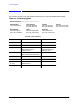
Contacting Agilent By internet, phone, or fax, get assistance with all your test and measurement needs. Table 1-1 Contacting Agilent Online assistance: www.agilent.
Safety Symbols The following safety symbols are used throughout this manual. Familiarize yourself with each of the symbols and its meaning before operating this instrument. Caution Caution denotes a hazard. It calls attention to a procedure that, if not correctly performed or adhered to, would result in damage to or destruction of the instrument. Do not proceed beyond a caution note until the indicated conditions are fully understood and met. Warning Warning denotes a hazard.
General Safety Considerations Warning This is a Safety Class I product (provided with a protective earthing ground incorporated in the power cord). The mains plug shall only be inserted in a socket outlet provided with a protective earth contact. Any interruption of the protective conductor, inside or outside the instrument, is likely to make the instrument dangerous. Intentional interruption is prohibited. Warning No operator serviceable parts inside. Refer servicing to quali ed personnel.
User's Guide Overview Chapter 1, \HP 8753D Description and Options," describes features, functions, and available options. Chapter 2, \Making Measurements," contains step-by-step procedures for making measurements or using particular functions. Chapter 3, \Making Mixer Measurements," contains step-by-step procedures for making calibrated and error-corrected mixer measurements.
Network Analyzer Documentation Set The Installation and Quick Start Guide familiarizes you with the network analyzer's front and rear panels, electrical and environmental operating requirements, as well as procedures for installing, con guring, and verifying the operation of the analyzer. The User's Guide shows how to make measurements, explains commonly-used features, and tells you how to get the most performance from your analyzer. The Quick Reference Guide provides a summary of selected user features.
x
Contents 1. HP 8753D Description and Options Where to Look for More Information . . . . . . . . . Analyzer Description . . . . . . . . . . . . . . . . . Front Panel Features . . . . . . . . . . . . . . . . . Analyzer Display . . . . . . . . . . . . . . . . . . Rear Panel Features and Connectors . . . . . . . . . Analyzer Options Available . . . . . . . . . . . . . . Option 1D5, High Stability Frequency Reference . . . Option 002, Harmonic Mode . . . . . . . . . . . . Option 006, 6 GHz Operation . . . . . .
To Title the Active Channel Display . . . . . . . . . . . . . . . . . . . Using Analyzer Display Markers . . . . . . . . . . . . . . . . . . . . . To Use Continuous and Discrete Markers . . . . . . . . . . . . . . . . To Activate Display Markers . . . . . . . . . . . . . . . . . . . . . . To Use Delta (1) Markers . . . . . . . . . . . . . . . . . . . . . . . . To Activate a Fixed Marker . . . . . . . . . . . . . . . . . . . . . . .
Creating a Sequence . . . . . . . . . . . . . . . . . . Running a Sequence . . . . . . . . . . . . . . . . . Stopping a Sequence . . . . . . . . . . . . . . . . . Editing a Sequence . . . . . . . . . . . . . . . . . Deleting Commands . . . . . . . . . . . . . . . . Inserting a Command . . . . . . . . . . . . . . . Modifying a Command . . . . . . . . . . . . . . . Clearing a Sequence from Memory . . . . . . . . . . Changing the Sequence Title . . . . . . . . . . . . . Naming Files Generated by a Sequence . .
4. Printing, Plotting, and Saving Measurement Results Where to Look for More Information . . . . . . . . . . . . . . . . . . Printing or Plotting Your Measurement Results . . . . . . . . . . . . . . Con guring a Print Function . . . . . . . . . . . . . . . . . . . . . . De ning a Print Function . . . . . . . . . . . . . . . . . . . . . . . If You are Using a Color Printer . . . . . . . . . . . . . . . . . . . . To Reset the Printing Parameters to Default Values . . . . . . . . . . .
ASCII Data Formats . . . . . . . . . . . . CITI le . . . . . . . . . . . . . . . . . S2P Data Format . . . . . . . . . . . . . Re-Saving an Instrument State . . . . . . . . Deleting a File . . . . . . . . . . . . . . . . To Delete an Instrument State File . . . . . To Delete all Files . . . . . . . . . . . . . Renaming a File . . . . . . . . . . . . . . . Recalling a File . . . . . . . . . . . . . . . Formatting a Disk . . . . . . . . . . . . . .
Using Continuous Correction Mode . . . . . . . . . . . . . . To Calibrate the Analyzer Receiver to Measure Absolute Power Matched Adapters . . . . . . . . . . . . . . . . . . . . . . Modify the Cal Kit Thru De nition . . . . . . . . . . . . . . Calibrating for Noninsertable Devices . . . . . . . . . . . . . . Adapter Removal . . . . . . . . . . . . . . . . . . . . . . Perform the 2-port Error Corrections . . . . . . . . . . . . Remove the Adapter . . . . . . . . . . . . . . . . . . . . Verify the Results .
Raw Arrays . . . . . . . . . . . . . . . . . . Vector Error-correction (Accuracy Enhancement) Trace Math Operation . . . . . . . . . . . . . Gating (Option 010 Only) . . . . . . . . . . . . The Electrical Delay Block . . . . . . . . . . . Conversion . . . . . . . . . . . . . . . . . . Transform (Option 010 Only) . . . . . . . . . . Format . . . . . . . . . . . . . . . . . . . . Smoothing . . . . . . . . . . . . . . . . . . . Format Arrays . . . . . . . . . . . . . . . . . O set and Scale . . . . . . . . . .
Understanding S-Parameters . . . . . . . . . . . . The S-Parameter Menu . . . . . . . . . . . . . . . Analog In Menu . . . . . . . . . . . . . . . . . Conversion Menu . . . . . . . . . . . . . . . . Input Ports Menu . . . . . . . . . . . . . . . . The Format Menu . . . . . . . . . . . . . . . . . . Log Magnitude Format . . . . . . . . . . . . . . . Phase Format . . . . . . . . . . . . . . . . . . . Group Delay Format . . . . . . . . . . . . . . . . Smith Chart Format . . . . . . . . . . . . . . . .
Calibration Considerations . . . . . . . . . . . . . . . . . . . . . . . . Measurement Parameters . . . . . . . . . . . . . . . . . . . . . . . . Device Measurements . . . . . . . . . . . . . . . . . . . . . . . . . Omitting Isolation Calibration . . . . . . . . . . . . . . . . . . . . . . Saving Calibration Data . . . . . . . . . . . . . . . . . . . . . . . . The Calibration Standards . . . . . . . . . . . . . . . . . . . . . . . Frequency Response of Calibration Standards . . . . . . . . . . . . . .
Power Sensor Calibration Factor List . . . . . . . . . . . . . . Speed and Accuracy . . . . . . . . . . . . . . . . . . . . . . Test Equipment Used . . . . . . . . . . . . . . . . . . . . Stimulus Parameters . . . . . . . . . . . . . . . . . . . . . Notes On Accuracy . . . . . . . . . . . . . . . . . . . . . . Alternate and Chop Sweep Modes . . . . . . . . . . . . . . . . Alternate . . . . . . . . . . . . . . . . . . . . . . . . . . . Chop . . . . . . . . . . . . . . . . . . . . . . . . . . . . .
Harmonic Operation (Option 002 only) . . . . . . . . . . . . . . . . . . . Typical Test Setup . . . . . . . . . . . . . . . . . . . . . . . . . . . . Single-Channel Operation . . . . . . . . . . . . . . . . . . . . . . . . . Dual-Channel Operation . . . . . . . . . . . . . . . . . . . . . . . . . Coupling Power Between Channels 1 and 2 . . . . . . . . . . . . . . . . Frequency Range . . . . . . . . . . . . . . . . . . . . . . . . . . . . Accuracy and input power . . . . . . . . . . . . . . . . . . . . . . .
Sequence Size . . . . . . . . . . . . . . . . . . . . . . . . . . . Embedding the Value of the Loop Counter In a Title . . . . . . . . . Autostarting Sequences . . . . . . . . . . . . . . . . . . . . . . The GPIO Mode . . . . . . . . . . . . . . . . . . . . . . . . . . The Sequencing Menu . . . . . . . . . . . . . . . . . . . . . . . . Gosub Sequence Command . . . . . . . . . . . . . . . . . . . . . . TTL I/O Menu . . . . . . . . . . . . . . . . . . . . . . . . . . . .
On-Wafer Measurements . . . . . . . . . . . . . . . . . . . . . . . . . . 7. Speci cations and Measurement Uncertainties Dynamic Range . . . . . . . . . . . . . . . . . . . . . . . . . HP 8753D Network Analyzer Speci cations . . . . . . . . . . . . HP 8753D (50 ) with 7 mm Test Ports . . . . . . . . . . . . . . Measurement Port Characteristics . . . . . . . . . . . . . . . Transmission Measurement Uncertainties . . . . . . . . . . . Re ection Measurement Uncertainties . . . . . . . . . . . .
Environmental Characteristics . . . General Conditions . . . . . . . . Operating Conditions . . . . . . . Non-Operating Storage Conditions Weight . . . . . . . . . . . . . . Cabinet Dimensions . . . . . . . . Internal Memory . . . . . . . . . . . . . . . . . . . . . . . . . . . . . . . . . . . . . . . . . . . . . . . . . . . . . . . . . . . . . . . . . . . . . . . . . . . . . . . . . . . . . . . . . . . . . . . . . . . . . . . . . . . . . . . . . . . . . . . . . . . . . . . . . . . . . . .
HPGL/2 Compatible Printer (used as a plotter) . Pen Plotter . . . . . . . . . . . . . . . . . If the Peripheral is a Power Meter . . . . . . . If the Peripheral is an External Disk Drive . . . If the Peripheral is a Computer Controller . . . . Con guring the Analyzer to Produce a Time Stamp HP-IB Programming Overview . . . . . . . . . . HP-IB Operation . . . . . . . . . . . . . . . . . Device Types . . . . . . . . . . . . . . . . . Talker . . . . . . . . . . . . . . . . . . . . Listener . . . . . . . . . .
The CITI le Keyword Reference . . . . . . . . . . . . . . . . . . . . . . .
Figures 1-1. 1-2. 1-3. 2-1. 2-2. 2-3. 2-4. 2-5. 2-6. 2-7. 2-8. 2-9. 2-10. 2-11. 2-12. 2-13. 2-14. 2-15. 2-16. 2-17. 2-18. 2-19. 2-20. 2-21. 2-22. 2-23. 2-24. 2-25. 2-26. 2-27. 2-28. 2-29. 2-30. 2-31. 2-32. 2-33. 2-34. 2-35. 2-36. 2-37. 2-38. 2-39. 2-40. 2-41. 2-42. HP 8753D Front Panel . . . . . . . . . . . . . . . . . . . . . . . . Analyzer Display (Single Channel, Cartesian Format) . . . . . . . . . . HP 8753D Rear Panel . . . . . . . . . . . . . . . . . . . . . . . . Basic Measurement Setup . . . . . .
2-43. 2-44. 2-45. 2-46. 2-47. 2-48. 2-49. 2-50. 2-51. 2-52. 2-53. 2-54. 2-55. 2-56. 3-1. 3-2. 3-3. 3-4. 3-5. 3-6. 3-7. 3-8. 3-9. 3-10. 3-11. 3-12. 3-13. 3-14. 3-15. 3-16. 3-17. 3-18. 3-19. 3-20. 3-21. 3-22. 3-23. 3-24. 3-25. 3-26. 3-27. 3-28. 3-29. 3-30. 4-1. 4-2. 4-3. 4-4. 4-5. 4-6. 4-7. 4-8. 4-9. 4-10. Gain Compression Using Power Sweep . . . . . . . . . . . . . . . . . . . Gain and Reverse Isolation . . . . . . . . . . . . . . . . . . . . . . . . . Typical Test Setup for Tuned Receiver Mode . . . . . .
4-11. Plot Quadrants . . . . . . . . . . . . . . . . . . . . . . . . . . . 4-12. Data Processing Flow Diagram . . . . . . . . . . . . . . . . . . . . 5-1. Standard Connections for a Response Error-Correction for Re ection Measurement . . . . . . . . . . . . . . . . . . . . . . . . . . . 5-2. Standard Connections for Response Error-Correction for Transmission Measurements . . . . . . . . . . . . . . . . . . . . . . . . . . 5-3. Standard Connections for Receiver Calibration . . . . . . . . . . . . . 5-4.
6-35. 6-36. 6-37. 6-38. 6-39. 6-40. 6-41. 6-42. 6-43. 6-44. 6-45. 6-46. 6-47. 6-48. 6-49. 6-50. 6-51. 6-52. 6-53. 6-54. 6-55. 6-56. 6-57. 6-58. 6-59. 6-60. 6-61. 6-62. 6-63. 6-64. 6-65. 6-66. 6-67. 6-68. 6-69. 6-70. 6-71. 6-72. 6-73. 6-74. 6-75. 6-76. 6-77. 6-78. 6-79. 6-80. 6-81. 6-82. 6-83. 6-84. Re ection Tracking ERF . . . . . . . . . . . . . . . . . . . . . . . . . . \Perfect Load" Termination . . . . . . . . . . . . . . . . . . . . . . . . Measured E ective Directivity . . . . . . . . . . . . . . . .
6-85. Swept Power Measurement of Ampli er's Fundamental Gain Compression and 2nd Harmonic Output Level . . . . . . . . . . . . . . . . . . . . . . . 6-86. Test Con guration for Setting RF Input using Automatic Power Meter Calibration 6-87. Mixer Parameters . . . . . . . . . . . . . . . . . . . . . . . . . . . . . 6-88. Conversion Loss versus Output Frequency Without Attenuators at Mixer Ports 6-89. Example of Conversion Loss versus Output Frequency Without Correct IF Signal Path Filtering . . . . . . . . .
Tables 0-1. 1-1. 2-1. 2-2. 4-1. 4-2. 4-3. 4-4. 4-5. 4-6. 4-7. 5-1. 5-2. 5-3. 5-4. 5-5. 5-6. 6-1. 6-2. 6-3. 6-4. 6-5. 6-6. 6-7. 6-8. 6-9. 6-10. 6-11. 6-12. 7-1. 7-2. 7-3. 7-4. 7-5. 7-6. 7-7. 7-8. 7-9. Hewlett-Packard Sales and Service O ces . . . . . . . . . . . . . . . . . . Comparing the HP 8753A/B/C/D . . . . . . . . . . . . . . . . . . . . . . Connector Care Quick Reference . . . . . . . . . . . . . . . . . . . . . . Gate Characteristics . . . . . . . . . . . . . . . . . . . . . . . . . . . .
7-10. Measurement Port Characteristics (Corrected)* for HP 8753D (75 ) using HP 85039A M-M Testports . . . . . . . . . . . . . . . . . . . . . . . . 7-11. Measurement Port Characteristics (Corrected)* for HP 8753D (75 ) using HP 85039A M-F Testports . . . . . . . . . . . . . . . . . . . . . . . . . 9-1. Cross Reference of Key Function to Programming Command . . . . . . . . 9-2. Softkey Locations . . . . . . . . . . . . . . . . . . . . . . . . . . . . 11-1. Code Naming Convention . . . . . . . . . . . . . .
1 HP 8753D Description and Options This chapter contains information on the following topics: Analyzer overview Analyzer description Front panel features Analyzer display Rear panel features and connectors Analyzer options available Service and support options Changes between the HP 8753 network analyzers Where to Look for More Information Additional information about many of the topics discussed in this chapter is located in the following areas: Chapter 2, \Making Measurements," contains step-by-step pro
Analyzer Description The HP 8753D is a high performance vector network analyzer for laboratory or production measurements of re ection and transmission parameters. It integrates a high resolution synthesized RF source, an S-parameter test set, and a dual channel three-input receiver to measure and display magnitude, phase, and group delay responses of active and passive RF networks.
Accuracy Accuracy enhancement methods that range from normalizing data to complete one or two port vector error correction with up to 1601 measurement points, and TRL*/LRM*. (Vector error correction reduces the e ects of system directivity, frequency response, source and load match, and crosstalk.) Power meter calibration that allows you to use an HP-IB compatible power meter to monitor and correct the analyzer's output power at each data point.
Front Panel Features Figure 1-1. HP 8753D Front Panel Figure 1-1 shows the location of the following front panel features and key function blocks. These features are described in more detail later in this chapter, and in Chapter 9, \Key De nitions." 1. LINE switch. This switch controls ac power to the analyzer. 1 is on, 0 is o . 2. Display. This shows the measurement data traces, measurement annotation, and softkey labels. The display is divided into speci c information areas, illustrated in Figure 1-2. 3.
7. 8. 9. 10. 11. 12. 13. The ENTRY block. This block includes the knob, the step 4*5 4+5 keys, and the number pad. These allow you to enter numerical data and control the markers. You can use the numeric keypad to select digits, decimal points, and a minus sign for numerical entries. You must also select a units terminator to complete value inputs. INSTRUMENT STATE function block.
Analyzer Display Figure 1-2. Analyzer Display (Single Channel, Cartesian Format) The analyzer display shows various measurement information: The grid where the analyzer plots the measurement data. The currently selected measurement parameters. The measurement data traces. Figure 1-2 illustrates the locations of the di erent information labels described below. In addition to the full-screen display shown in Figure 1-2, a split display is available, as described in Chapter 2, \Making Measurements.
2. Stimulus Stop Value. This value could be any one of the following: The stop frequency of the source in frequency domain measurements. The stop time in time domain measurements or CW sweeps. The upper limit of a power sweep. When the stimulus is in center/span mode, the span is shown in this space. The stimulus values can be blanked, as described under \ FREQUENCY BLANK Key" in Chapter 9, \Key De nitions.
H=2 = Harmonic mode is on, and the second harmonic is being measured (harmonics Option 002 only). See \Analyzer Options Available" later in this chapter.) H=3 = Harmonic mode is on, and the third harmonic is being measured (harmonics Option 002 only). (See \Analyzer Options Available" later in this chapter.) Hld = Hold sweep. (See HOLD in Chapter 9, \Key De nitions.") NNNNNNNNNNNNNN man = Waiting for manual trigger. PC = Power meter calibration is on.
11. Reference Level. This value is the reference line in Cartesian formats or the outer circle in polar formats, whichever you selected using the 4SCALE REF5 key. The reference level is also indicated by a small triangle adjacent to the graticule, at the left for channel 1 and at the right for channel 2 in Cartesian formats. 12. Marker Values. These are the values of the active marker, in units appropriate to the current measurement.
Rear Panel Features and Connectors Figure 1-3. HP 8753D Rear Panel Figure 1-3 illustrates the features and connectors of the rear panel, described below. Requirements for input signals to the rear panel connectors are provided in Chapter 7, \Speci cations and Measurement Uncertainties." 1. Serial number plate. The serial number of the instrument is located on this plate. 2.
10. 10 MHZ PRECISION REFERENCE OUTPUT. (Option 1D5) 11. EXTERNAL REFERENCE INPUT connector. This allows for a frequency reference signal input that can phase lock the analyzer to an external frequency standard for increased frequency accuracy. The analyzer automatically enables the external frequency reference feature when a signal is connected to this input. When the signal is removed, the analyzer automatically switches back to its internal frequency reference. 12. AUXILIARY INPUT connector.
Analyzer Options Available Option 1D5, High Stability Frequency Reference Option 1D5 o ers 60.05 ppm temperature stability from 0 to 60 C (referenced to 25 C). Option 002, Harmonic Mode Provides measurement of second or third harmonics of the test device's fundamental output signal. Frequency and power sweep are supported in this mode. Harmonic frequencies can be measured up to the maximum frequency of the receiver. However, the fundamental frequency may not be lower than 16 MHz.
Service and Support Options The analyzer automatically includes a one-year on-site service warranty, where available. The following service and support products are available with an HP 8753D network analyzer at any time during or after the time of purchase. Additional service and support options may be available at some sites. Consult your local HP customer engineer for details.
Changes between the HP 8753 Network Analyzers Table 1-1. Comparing the HP 8753A/B/C/D Feature 8753A 8753B 8753C 8753D Fully integrated measurement system (built-in No No No Yes test set) y y y +10 to 085 Test port power range (dBm) No No No Yes Auto/manual power range selecting No No No Yes Port power coupling/uncoupling No No No Yes Internal disk drive No No No Yes Precision frequency reference (Option 1D5) 300 kHz 300 kHz 300 kHz 30 kHz Frequency range - low end No Yes Yes Yes Ext. freq.
2 Making Measurements This Chapter contains the following example procedures for making measurements or using particular functions: Basic measurement sequence and example Setting frequency range Setting source power Analyzer display functions Analyzer marker functions Magnitude and insertion phase response Electrical length and phase distortion Deviation from linear phase Group delay Limit testing Gain compression Gain and reverse isolation High Power Measurements Tuned Receiver Mode Test sequencing Time do
Principles of Microwave Connector Care Proper connector care and connection techniques are critical for accurate, repeatable measurements. Refer to the calibration kit documentation for connector care information. Prior to making connections to the network analyzer, carefully review the information about inspecting, cleaning and gaging connectors. Having good connector care and connection techniques extends the life of these devices. In addition, you obtain the most accurate measurements.
Basic Measurement Sequence and Example Basic Measurement Sequence There are ve basic steps when you are making a measurement. 1. Connect the device under test and any required test equipment. Caution 2. 3. 4. 5. Damage may result to the device under test if it is sensitive to analyzer's default output power level. To avoid damaging a sensitive DUT, perform step 2 before step 1. Choose the measurement parameters. Perform and apply the appropriate error-correction. Measure the device under test.
4. To set the span to 30 MHz, press: 4SPAN5 4305 4M/ 5 Note You could also press the 4START5 and 4STOP5 keys and enter the frequency range limits as start frequency and stop frequency values. Setting the Source Power. 5.
Using the Display Functions To View Both Measurement Channels In some cases, you may want to view more than one measured parameter at a time. Simultaneous gain and phase measurements for example, are useful in evaluating stability in negative feedback ampli ers. You can easily make such measurements using the dual channel display. 1. To see both channels simultaneously, press: 4DISPLAY5 NNNNNNNNNNNNNNNNNNNNNNNNNNNNNNNNNNNNNN DUAL CHAN ON Figure 2-2.
2. You can view the measurements on separate displays, press: MORE SPLIT DISP ON The analyzer shows channel 1 on the upper half of the display and channel 2 on the lower half of the display. The analyzer also defaults to measuring S11 on channel 1 and S21 on channel 2. NNNNNNNNNNNNNN NNNNNNNNNNNNNNNNNNNNNNNNNNNNNNNNNNNNNNNNN Figure 2-3. Example Dual Channel With Split Display On 3.
To Divide Measurement Data by the Memory Trace You can use this feature for ratio comparison of two traces, for example, measurements of gain or attenuation. 1. You must have already stored a data trace to the active channel memory, as described in \To Save a Data Trace to the Display Memory." 2. Press 4DISPLAY5 DATA/MEM to divide the data by the memory. NNNNNNNNNNNNNNNNNNNNNNNNNN The analyzer normalizes the data to the memory, and shows the results.
To Title the Active Channel Display 1. Press 4DISPLAY5 MORE TITLE to access the title menu. NNNNNNNNNNNNNN NNNNNNNNNNNNNNNNN 2. Press ERASE TITLE and enter the title you want for your measurement display. NNNNNNNNNNNNNNNNNNNNNNNNNNNNNNNNNNN If you have a DIN keyboard attached to the analyzer, type the title you want from the keyboard. Then press 4ENTER5 to enter the title into the analyzer. You can enter a title that has a maximum of 50 characters.
Using Analyzer Display Markers The analyzer markers provide numerical readout of trace data. You can control the marker search, the statistical functions, and the capability for quickly changing stimulus parameters with markers, from the 4MARKER FCTN5 key. Markers have a stimulus value (the x-axis value in a Cartesian format) and a response value (the y-axis value in a Cartesian format).
To Activate Display Markers To switch on marker 1 and make it the active marker, press: 4MARKER5 NNNNNNNNNNNNNNNNNNNNNNNNNN MARKER 1 The active marker appears on the analyzer display as r. The active marker stimulus value is displayed in the active entry area. You can modify the stimulus value of the active marker, using the front panel knob or numerical keypad. All of the marker response and stimulus values are displayed in the upper right corner of the display. Figure 2-5.
To switch o all of the markers, press: NNNNNNNNNNNNNNNNNNNNNNN ALL OFF To Use Delta (1) Markers This is a relative mode, where the marker values show the position of the active marker relative to the delta reference marker. You can switch on the delta mode by de ning one of the ve markers as the delta reference. 1. Press 4MARKER5 1 MODE MENU 1 REF=1 to make marker 1 a reference marker. NNNNNNNNNNNNNNNNNNNNNNNNNNNNNNNNNNN NNNNNNNNNNNNNNNNNNNNNNN 2.
Using the 1REF=1FIXED NNNNNNNNNNNNNNNNNNNNNNNNNNNNNNNNNNNNNNNNNNNNNNNNNNN MKR Key to activate a Fixed Reference Marker 1.
Using the MKR NNNNNNNNNNNNNNNNNNNNNNNNNNNN ZERO Key to Activate a Fixed Reference Marker Marker zero enters the position of the active marker as the 1 reference position. Alternatively, you can specify the xed point with FIXED MKR POSITION . Marker zero is canceled by switching delta mode o . 1. To place marker 1 at a point that you would like to reference, press: 4MARKER5 and turn the front panel knob or enter a value from the front panel keypad. 2.
To Couple and Uncouple Display Markers At a preset state, the markers have the same stimulus values on each channel, but they can be uncoupled so that each channel has independent markers. 1. Press 4MARKER FCTN5 MARKER MODE MENU and select from the following keys: NNNNNNNNNNNNNNNNNNNNNNNNNNNNNNNNNNNNNNNNNNNNNNNNNN NNNNNNNNNNNNNNNNNNNNNNNNNNNNNNNNNNNNNNNNNNNNNNNNNN Choose MARKERS: COUPLED if you want the analyzer to couple the marker stimulus values for the two display channels.
2. Select the type of polar marker you want from the following choices: NNNNNNNNNNNNNNNNNNNNNNN Choose LIN MKR if you want to view the magnitude and the phase of the active marker. The magnitude values appear in units and the phase values appear in degrees. NNNNNNNNNNNNNNNNNNNNNNN Choose LOG MKR if you want to view the logarithmic magnitude and the phase of the active marker. The magnitude values appear in dB and the phase values appear in degrees.
The marker annotation tells that the complex impedance is capacitive in the bottom half of the Smith chart display and is inductive in the top half of the display. NNNNNNNNNNNNNNNNNNNNNNN Choose LIN MKR if you want the analyzer to show the linear magnitude and the phase of the re ection coe cient at the marker. Choose LOG MKR if you want the analyzer to show the logarithmic magnitude and the phase of the re ection coe cient at the active marker.
Setting the Start Frequency 1. Press 4MARKER FCTN5 and turn the front panel knob or enter a value from the front panel keypad to position the marker at the value that you want for the start frequency. 2. Press MARKER!START to change the start frequency value to the value of the active marker. NNNNNNNNNNNNNNNNNNNNNNNNNNNNNNNNNNNNNNNN Figure 2-13. Example of Setting the Start Frequency Using a Marker Setting the Stop Frequency 1.
Setting the Center Frequency 1. Press 4MARKER FCTN5 and turn the front panel knob or enter a value from the front panel keypad to position the marker at the value that you want for the center frequency. 2. Press MARKER!CENTER to change the center frequency value to the value of the active marker. NNNNNNNNNNNNNNNNNNNNNNNNNNNNNNNNNNNNNNNNNNN Figure 2-15.
Setting the Frequency Span You can set the span equal to the spacing between two markers. If you set the center frequency before you set the frequency span, you will have a better view of the area of interest. 1. Press 4MARKER5 1MODE MENU 1REF=1 MARKER 2 . NNNNNNNNNNNNNNNNNNNNNNNNNNNNNNNN NNNNNNNNNNNNNNNNNNNN NNNNNNNNNNNNNNNNNNNNNNNNNN 2. Turn the front panel knob or enter a value from the front panel keypad to position the markers where you want the frequency span.
Setting the Display Reference Value 1. Press 4MARKER FCTN5 and turn the front panel knob or enter a value from the front panel keypad to position the marker at the value that you want for the analyzer display reference value. 2. Press MARKER!REFERENCE to change the reference value to the value of the active marker. NNNNNNNNNNNNNNNNNNNNNNNNNNNNNNNNNNNNNNNNNNNNNNNNNNNN Figure 2-17.
Setting the Electrical Delay This feature adds phase delay to a variation in phase versus frequency, therefore it is only applicable for ratioed inputs. 1. Press 4FORMAT5 PHASE . NNNNNNNNNNNNNNNNN 2. Press 4MARKER FCTN5 and turn the front panel knob or enter a value from the front panel keypad to position the marker at a point of interest. 3. Press MARKER!DELAY to automatically add or subtract enough line length to the receiver input to compensate for the phase slope at the active marker position.
To Search for a Speci c Amplitude These functions place the marker at an amplitude-related point on the trace. If you switch on tracking, the analyzer searches every new trace for the target point. Searching for the Maximum Amplitude 1. Press 4MARKER FCTN5 MKR SEARCH to access the marker search menu. NNNNNNNNNNNNNNNNNNNNNNNNNNNNNNNN 2. Press SEARCH: MAX to move the active marker to the maximum point on the measurement trace. NNNNNNNNNNNNNNNNNNNNNNNNNNNNNNNNNNN Figure 2-19.
Searching for the Minimum Amplitude 1. Press 4MARKER FCTN5 MKR SEARCH to access the marker search menu. NNNNNNNNNNNNNNNNNNNNNNNNNNNNNNNN 2. Press SEARCH: MIN to move the active marker to the minimum point on the measurement trace. NNNNNNNNNNNNNNNNNNNNNNNNNNNNNNNNNNN Figure 2-20.
Searching for a Target Amplitude 1. Press 4MARKER FCTN5 MKR SEARCH to access the marker search menu. NNNNNNNNNNNNNNNNNNNNNNNNNNNNNNNN 2. Press SEARCH: TARGET to move the active marker to the target point on the measurement trace. 3. If you want to change the target amplitude value (default is 03 dB), press TARGET and enter the new value from the front panel keypad. 4. If you want to search for multiple responses at the target amplitude value, press SEARCH LEFT and SEARCH RIGHT .
Searching for a Bandwidth The analyzer can automatically calculate and display the 03 dB bandwidth (BW:), center frequency (CENT:), Q, and loss of the device under test at the center frequency. (Q stands for \quality factor," de ned as the ratio of a circuit's resonant frequency to its bandwidth.) These values are shown in the marker data readout. 1. Press 4MARKER5 and turn the front panel knob or enter a value from the front panel keypad to place the marker at the center of the lter passband. 2.
To Calculate the Statistics of the Measurement Data This function calculates the mean, standard deviation, and peak-to-peak values of the section of the displayed trace between the active marker and the delta reference. If there is no delta reference, the analyzer calculates the statistics for the entire trace. 1. Press 4MARKER5 1 MODE MENU 1 REF=1 to make marker 1 a reference marker. NNNNNNNNNNNNNNNNNNNNNNNNNNNNNNNNNNN NNNNNNNNNNNNNNNNNNNNNNN 2.
Measuring Magnitude and Insertion Phase Response The analyzer allows you to make two di erent measurements simultaneously. You can make these measurements in di erent formats for the same parameter. For example, you could measure both the magnitude and phase of transmission. You could also measure two di erent parameters (S11 and S22 ).
4. Reconnect your test device. 5. To better view the measurement trace, press: 4SCALE NNNNNNNNNNNNNNNNNNNNNNNNNNNNNNNN REF5 AUTO SCALE 6. To locate the maximum amplitude of the device response, as shown in Figure 2-25, press: 4MARKER NNNNNNNNNNNNNNNNNNNNNNNNNNNNNNNN NNNNNNNNNNNNNNNNNNNNNNNNNNNNNNNNNNN FCTN5 MKR SEARCH SEARCH: MAX Figure 2-25. Example Magnitude Response Measurement Results Measuring Insertion Phase Response 7.
The phase response shown in Figure 2-27 is undersampled; that is, there is more than 180 phase delay between frequency points. If the 1 = >180 , incorrect phase and delay information may result. Figure 2-27 shows an example of phase samples being with 1 less than 180 and greater than 180 . Figure 2-27. Phase Samples Undersampling may arise when measuring devices with long electrical length.
Measuring Electrical Length and Phase Distortion Electrical Length The analyzer mathematically implements a function similar to the mechanical \line stretchers" of earlier analyzers. This feature simulates a variable length lossless transmission line, which you can add to or remove from the analyzer's receiver input to compensate for interconnecting cables, etc. In this example, the electronic line stretcher measures the electrical length of a SAW lter.
3. Substitute a thru for the device and perform a response calibration by pressing: 4CAL5 NNNNNNNNNNNNNNNNNNNNNNNNNNNNNNNNNNNNNNNNNNNN NNNNNNNNNNNNNNNNNNNNNNNNNN NNNNNNNNNNNNNN CALIBRATE MENU RESPONSE THRU 4. Reconnect your test device. 5. To better view the measurement trace, press: 4SCALE NNNNNNNNNNNNNNNNNNNNNNNNNNNNNNNN REF5 AUTO SCALE Notice that in Figure 2-29 the SAW lter under test has considerable phase shift within only a 2 MHz span.
8. Press 4SCALE REF5 ELECTRICAL DELAY and turn the front panel knob to increase the electrical length until you achieve the best at line, as shown in Figure 2-30. The measurement value that the analyzer displays represents the electrical length of your device relative to the speed of light in free space. The physical length of your device is related to this value by the propagation velocity of its medium.
1. Follow the procedure in \Measuring Electrical Length." 2. To increase the scale resolution, press: NNNNNNNNNNNNNNNNNNNNNNNNNNNNN and turn the front panel knob or enter a value from the front panel keypad. 3. To use the marker statistics to measure the maximum peak-to-peak deviation from linear phase, press: 4SCALE REF5 SCALE DIV 4MARKER NNNNNNNNNNNNNNNNNNNNNNNNNNNNNNNNNNNNNNNNN NNNNNNNNNNNNNNNNNNNNNNNNNN FCTN5 MKR MODE MENU STATS ON 4.
3. To activate a marker to measure the group delay at a particular frequency, press: 4MARKER5 and turn the front panel knob or enter a value from the front panel keypad. Figure 2-32. Group Delay Example Measurement Group delay measurements may require a speci c aperture (1f) or frequency spacing between measurement points. The phase shift between two adjacent frequency points must be less than 180 , otherwise incorrect group delay information may result. 4.
5. To increase the e ective group delay aperture, by increasing the number of measurement points over which the analyzer calculates the group delay, press: NNNNNNNNNNNNNNNNNNNNNNNNNNNNNNNNNNNNNNNNNNNNNNNNNNNNNNNN SMOOTHING APERTURE 455 4x15 As the aperture is increased the \smoothness" of the trace improves markedly, but at the expense of measurement detail. Figure 2-34.
Testing A Device with Limit Lines Limit testing is a measurement technique that compares measurement data to constraints that you de ne. Depending on the results of this comparison, the analyzer will indicate if your device either passes or fails the test. Limit testing is implemented by creating individual at, sloping, and single point limit lines on the analyzer display. When combined, these lines can represent the performance parameters for your device under test.
4. Reconnect your test device. 5.
5. To terminate the at line segment by establishing a single point limit, press: NNNNNNNNNNN ADD STIMULUS VALUE 41405 4M/ 5 DONE LIMIT TYPE SINGLE POINT RETURN NNNNNNNNNNNNNNNNNNNNNNNNNNNNNNNNNNNNNNNNNNNN NNNNNNNNNNNNNN NNNNNNNNNNNNNNNNNNNNNNNNNNNNNNNN NNNNNNNNNNNNNNNNNNNNNNNNNNNNNNNNNNNNNN NNNNNNNNNNNNNNNNNNNN Figure 2-36 shows the at limit lines that you have just created with the following parameters: stimulus from 127 MHz to 140 MHz upper limit of 021 dB lower limit of 027 dB Figure 2-36.
7.
3. To terminate the lines and create a sloping limit line, press: NNNNNNNNNNN ADD STIMULUS VALUE 41255 4M/ 5 UPPER LIMIT 40265 4x15 LOWER LIMIT 402005 4x15 DONE LIMIT TYPE SINGLE POINT RETURN NNNNNNNNNNNNNNNNNNNNNNNNNNNNNNNNNNNNNNNNNNNN NNNNNNNNNNNNNNNNNNNNNNNNNNNNNNNNNNN NNNNNNNNNNNNNNNNNNNNNNNNNNNNNNNNNNN NNNNNNNNNNNNNN NNNNNNNNNNNNNNNNNNNNNNNNNNNNNNNN NNNNNNNNNNNNNNNNNNNNNNNNNNNNNNNNNNNNNN NNNNNNNNNNNNNNNNNNNN 4.
Creating Single Point Limits In this example procedure, the following limits are set: from 023 dB to 028.5 dB at 141 MHz from 023 dB to 028.5 dB at 126.5 MHz 1. To access the limits menu and activate the limit lines, press: 4SYSTEM5 NNNNNNNNNNNNNNNNNNNNNNNNNNNNNNNN NNNNNNNNNNNNNNNNNNNNNNNNNNNNNNNNNNNNNNNNN NNNNNNNNNNNNNNNNNNNNNNNNNNNNNNNNNNNNNNNNNNNNNNN NNNNNNNNNNNNNNNNNNNNNNNNNNNNNNNN NNNNNNNNNNN LIMIT MENU LIMIT LINE ON EDIT LIMIT LINE CLEAR LIST YES 2.
Editing Limit Segments This example shows you how to edit the upper limit of a limit line. 1. To access the limits menu and activate the limit lines, press: 4SYSTEM5 NNNNNNNNNNNNNNNNNNNNNNNNNNNNNNNN NNNNNNNNNNNNNNNNNNNNNNNNNNNNNNNNNNNNNNNNN NNNNNNNNNNNNNNNNNNNNNNNNNNNNNNNNNNNNNNNNNNNNNNN LIMIT MENU LIMIT LINE ON EDIT LIMIT LINE 2.
Running a Limit Test 1. To access the limits menu and activate the limit lines, press: 4SYSTEM5 NNNNNNNNNNNNNNNNNNNNNNNNNNNNNNNN NNNNNNNNNNNNNNNNNNNNNNNNNNNNNNNNNNNNNNNNN NNNNNNNNNNNNNNNNNNNNNNNNNNNNNNNNNNNNNNNNNNNNNNN LIMIT MENU LIMIT LINE ON EDIT LIMIT LINE Reviewing the Limit Line Segments The limit table data that you have previously entered is shown on the analyzer display. 2.
O setting Limit Lines The limit o set functions allow you to adjust the limit lines to the frequency and output level of your device. For example, you could apply the stimulus o set feature for testing tunable lters. Or, you could apply the amplitude o set feature for testing variable attenuators, or passband ripple in lters with variable loss. This example shows you the o set feature and the limit test failure indications that can appear on the analyzer display. 1.
Measuring Gain Compression Gain compression occurs when the input power of an ampli er is increased to a level that reduces the gain of the ampli er and causes a nonlinear increase in output power. The point at which the gain is reduced by 1 dB is called the 1 dB compression point. The gain compression will vary with frequency, so it is necessary to nd the worst case point of gain compression in the frequency band.
b. To uncouple the channel stimulus so that the channel power will be uncoupled, press: 4MENU5 NNNNNNNNNNNNNNNNNNNNNNNNNNNNNNNNNNNNNNNNNNNN COUPLED CH OFF This will allow you to separately increase the power for channel 2 and channel 1, so that you can observe the gain compression on channel 2 while channel 1 remains unchanged. c.
14. To set the CW frequency before going into the power sweep mode, press: 4SEQ5 ! NNNNNNNNNNNNNNNNNNNNNNNNNNNNNNNNNNNNNNNNNNNNNNNNNNNNN NNNNNNNNNNNNNNNNNNNNNNNNNNNNNNNNNNNNN SPECIAL FUNCTIONS MARKER CW 15. Press 4MENU5 SWEEP TYPE MENU POWER SWEEP . NNNNNNNNNNNNNNNNNNNNNNNNNNNNNNNNNNNNNNNNNNNNNNN NNNNNNNNNNNNNNNNNNNNNNNNNNNNNNNNNNN 16. Enter the start and stop power levels for the sweep. Now channel 1 is displaying a gain compression curve. (Do not pay attention to channel 2 at this time.) 17.
Figure 2-43.
Measuring Gain and Reverse Isolation Simultaneously Since an ampli er will have high gain in the forward direction and high isolation in the reverse direction, the gain (S21 ) will be much greater than the reverse isolation (S12 ). Therefore, the power you apply to the input of the ampli er for the forward measurement (S21 ) should be considerably lower than the power you apply to the output for the reverse measurement (S12 ).
Note To obtain best accuracy, you should set the power levels prior to performing the calibration. However, the analyzer compensates for nominal power changes you make during a measurement, so that the error correction still remains approximately valid. In these cases, the Cor annunciator will change to C?. Figure 2-44.
Measurements Using the Tuned Receiver Mode In the tuned receiver mode, the analyzer's receiver operates independently of any signal source. This mode is not phase-locked and functions in all sweep types. The analyzer tunes the receiver to a synthesized CW input signal at a precisely speci ed frequency. All phase lock routines are bypassed, increasing sweep speed signi cantly. The external source must be synthesized, and must drive the analyzer's external frequency reference.
External Source Requirements An analyzer in tuned receiver mode can receive input signals into PORT 1, PORT 2, or R CHANNEL IN. Input power range speci cations are provided in Chapter 7, \Speci cations and Measurement Uncertainties.
Test Sequencing Test sequencing allows you to automate repetitive tasks. As you make a measurement, the analyzer memorizes the keystrokes. Later you can repeat the entire sequence by pressing a single key. Because the sequence is de ned with normal measurement keystrokes, you do not need additional programming expertise. Subroutines and limited decision-making increases the exibility of test sequences.
Creating a Sequence 1. To enter the sequence creation mode, press: 4SEQ5 d NNNNNNNNNNNNNNNNNNNNNNNNNNNNNNNNNNNNNNNNNNNNNNNNNNNNNNNN NEW SEQ/MODIFY SEQ As shown in Figure 2-46, a list of instructions appear on the analyzer display to help you create or edit a sequence. c a b Figure 2-46. Test Sequencing Help Instructions 2. To select a sequence position in which to store your sequence, press: NNNNNNNNNNNNNNNNNNNNNNNNNNNNNNNNNNNNNNNNNNNNNNN SEQUENCE 1 SEQ1 This choice selects sequence position #1.
3. To create a test sequence, enter the parameters for the measurement that you wish to make.
Editing a Sequence Deleting Commands 1. To enter the creation/editing mode, press: 4SEQ5 NNNNNNNNNNNNNNNNNNNNNNNNNNNNNNNNNNNNNNNNNNNNNNNNNNNNNNNN NEW SEQ/MODIFY SEQ 2. To select the particular test sequence you wish to modify (sequence 1 in this example), press: NNNNNNNNNNNNNNNNNNNNNNNNNNNNNNNNNNNNNNNNNNNNNNN SEQUENCE 1 SEQ1 3.
Modifying a Command 1. To enter the creation/editing mode, press: 4PRESET5 4SEQ5 NNNNNNNNNNNNNNNNNNNNNNNNNNNNNNNNNNNNNNNNNNNNNNNNNNNNNNNN NEW SEQ/MODIFY SEQ 2. To select the particular test sequence you wish to modify, (sequence 1 in this example), press: NNNNNNNNNNNNNNNNNNNNNNNNNNNNNNNNNNNNNNNNNNNNNNN SEQUENCE 1 SEQ1 The following list is the commands entered in \Creating a Sequence." Notice that for longer sequences, only a portion of the list can appear on the screen at one time.
Changing the Sequence Title If you are storing sequences on a disk, you should replace the default titles (SEQ1, SEQ2 . . . ). 1. To select a sequence that you want to retitle, press: 4SEQ5 NNNNNNNNNNNNNN NNNNNNNNNNNNNNNNNNNNNNNNNNNNNNNNNNNNNNNNNNNNNNN MORE TITLE SEQUENCE and select the particular sequence softkey. The analyzer shows the available title characters. The current title is displayed in the upper-left corner of the screen. 2.
Storing a Sequence on a Disk 1. To format a disk, refer to Chapter 4, \Printing, Plotting, and Saving Measurement Results." 2. To save a sequence to the internal disk, press: 4SEQ5 NNNNNNNNNNNNNN NNNNNNNNNNNNNNNNNNNNNNNNNNNNNNNNNNNNNNNNNNNNNNNNNNNNN MORE STORE SEQ TO DISK and select the particular sequence softkey. The disk drive access light should turn on brie y. When it goes out, the sequence has been saved. Caution The analyzer will overwrite a le on the disk that has the same title.
Loading a Sequence from Disk For this procedure to work, the desired le must exist on the disk in the analyzer drive. 1.
Cascading Multiple Example Sequences By cascading test sequences, you can create subprograms for a larger test sequence. You can also cascade sequences to extend the length of test sequences to greater than 200 lines. In this example, you are shown two sequences that have been cascaded. You can do this by having the last command in sequence 1 call sequence position 2, regardless of the sequence title.
Loop Counter Example Sequence This example shows you the basic steps necessary for constructing a looping structure within a test sequence. A typical application of this loop counter structure is for repeating a speci c measurement as you step through a series of CW frequencies or dc bias levels. For an example application, see \Fixed IF Mixer Measurements" in Chapter 3. 1.
Generating Files in a Loop Counter Example Sequence This example shows how to increment the names of tiles that are generated by a sequence with a loop structure.
Start of Sequence FILE NAME DT[LOOP] PLOT NAME PL[LOOP] SINGLE SAVE FILE 0 PLOT DECR LOOP COUNTER IF LOOP COUNTER 0 THEN DO SEQUENCE 2 Sequence 1 initializes the loop counter and calls sequence 2. Sequence 2 repeats until the loop counter reaches 0. It takes a single sweep, saves the data le and plots the display. The data le names generated by this sequence will be: DT00007.D1 through DT000001.D1 The plot le names generated by this sequence will be: PL00007.FP through PL00001.
RECALL REG 1 IF LIMIT TEST PASS THEN DO SEQUENCE 2 IF LIMIT TEST FAIL THEN DO SEQUENCE 3 2.
Measuring Swept Harmonics The analyzer has the unique capability of measuring swept second and third harmonics as a function of frequency in a real-time manner. Figure 2-47 displays the absolute power of the fundamental and second harmonic in dBm. Figure 2-48 shows the second harmonic's power level relative to the fundamental power in dBc. Follow the steps listed below to perform these measurements. 1.
Figure 2-48.
Measuring a Device in the Time Domain (Option 010 Only) The HP 8753D Option 010 allows you to measure the time domain response of a device. Time domain analysis is useful for isolating a device problem in time or in distance. Time and distance are related by the velocity factor of your device under test. The analyzer measures the frequency response of your device and uses an inverse Fourier transform to convert the data to the time domain.
2. To choose the measurement parameters, press: 4PRESET5 4MEAS5 NNNNNNNNNNNNNNNNNNNNNNNNNNNNNNNNNNNNNNNNNNNNNNNNNNNNNNNNNNN Trans:FWD S21 (B/R) 4START5 41195 4M/ 5 4STOP5 41495 4M/ 5 4SCALE NNNNNNNNNNNNNNNNNNNNNNNNNNNNNNNN REF5 AUTO SCALE 3. Substitute a thru for the device under test and perform a frequency response correction. Refer to \Calibrating the Analyzer," located at the beginning of this Chapter, for a detailed procedure. 4. Reconnect your device under test. 5.
8. To access the gate function menu, press: 4SYSTEM5 NNNNNNNNNNNNNNNNNNNNNNNNNNNNNNNNNNNNNNNNNNNN NNNNNNNNNNNNNNNNNNNNNNNNNNNNNNNNNNNNNN NNNNNNNNNNNNNNNNNNNN TRANSFORM MENU SPECIFY GATE CENTER 9. To set the gate parameters, by entering the marker value, press: 41.65 4M/ 5, or turn the front panel knob to position the \>" center gate marker. 10. To set the gate span, press: NNNNNNNNNNNNNN SPAN 41.25 4M/ 5 or turn the front panel knob to position the \ ag" gate markers. 11.
Table 2-2. Gate Characteristics Gate Shape Passband Ripple Sidelobe Levels Cuto Time Minimum Gate Span Gate Span Minimum 60.1 dB 60.1 dB 60.1 dB 60.01 dB 048 dB 068 dB 057 dB 070 dB 1.4/Freq Span 2.8/Freq Span 2.8/Freq Span 5.6/Freq Span 4.4/Freq Span 8.8/Freq Span 12.7/Freq Span 25.4/Freq Span Normal Wide Maximum NOTE: With 1601 frequency points, gating is available only in the bandpass mode. The passband ripple and sidelobe levels are descriptive of the gate shape.
Figure 2-53.
Re ection Response in Time Domain The time domain response of a re ection measurement is often compared with the time domain re ectometry (TDR) measurements. Like the TDR, the analyzer measures the size of the re ections versus time (or distance). Unlike the TDR, the time domain capability of the analyzer allows you to choose the frequency range over which you would like to make the measurement. 1.
4. To better view the measurement trace, press: 4SCALE NNNNNNNNNNNNNNNNNNNNNNNNNNNNNNNN REF5 AUTO SCALE Figure 2-55 shows the frequency domain re ection response of the cables under test. The complex ripple pattern is caused by re ections from the adapters interacting with each other. By transforming this data to the time domain, you can determine the magnitude of the re ections versus distance along the cable. Figure 2-55. Device Response in the Frequency Domain 5.
7. To enter the relative velocity of the cable under test, press: NNNNNNNNNNNNNN NNNNNNNNNNNNNNNNNNNNNNNNNNNNNNNNNNNNNNNNNNNNNNN MORE VELOCITY FACTOR and enter a velocity factor for your cable under test. 4CAL5 Note Most cables have a relative velocity of 0.66 (for polyethylene dielectrics) or 0.7 (for te on dielectrics). If you would like the markers to read actual one-way distance rather than return trip distance, enter one-half the actual velocity factor.
Non-coaxial Measurements The capability of making non-coaxial measurements is available with the HP 8753 family of analyzers with TRL* (thru-re ect-line) or LRM* (line-re ect-match) calibration. For indepth information on TRL*/LRM* calibration, refer to Chapter 6, \Application and Operation Concepts.
3 Making Mixer Measurements This chapter contains information and example procedures on the following topics: Measurement considerations Minimizing Source and Load Mismatches Reducing the E ect of Spurious Responses Eliminating Unwanted Mixing and Leakage Signals How RF and IF Are De ned Frequency O set Mode Operation Di erences Between Internal and External R-Channel Inputs Power Meter Calibration Conversion loss using the frequency o set mode High dynamic range swept RF/IF conversion loss Fixed IF measure
Measurement Considerations To ensure successful mixer measurements, the following measurement challenges must be taken into consideration: Mixer Considerations Minimizing Source and Load Mismatches Reducing the E ect of Spurious Responses Eliminating Unwanted Mixing and Leakage Signals Analyzer Operation How RF and IF Are De ned Frequency O set Mode Operation Di erences Between Internal and External R-Channel Inputs Power Meter Calibration Minimizing Source and Load Mismatches When characterizing linear d
NNNNNNNNNNNNNNNNNNNNNNNNNNNNNNNNNNNNNNNNNNNN In a down converter measurement where the DOWN CONVERTER softkey is selected, the notation on the analyzer's setup diagram indicates that the analyzer's source frequency is labeled RF, connecting to the mixer RF port, and the analyzer's receiver frequency is labeled IF, connecting to the mixer IF port. Because the RF frequency can be greater or less than the set LO frequency in this type of measurement, you can select either RF > LO or RF < LO .
Frequency O set Mode Operation Frequency o set measurements do not begin until all of the frequency o set mode parameters are set. These include the following: Start and Stop IF Frequencies LO frequency Up Converter / Down Converter RF > LO / RF < LO The LO frequency for frequency o set mode must be set to the same value as the external LO source. The o set frequency between the analyzer source and receiver will be set to this value.
3. To activate the frequency o set mode, press: 4SYSTEM 5 NNNNNNNNNNNNNNNNNNNNNNNNNNNNNNNNNNNNNNNNNNNNNNN INSTRUMENT MODE NNNNNNNNNNNNNNNNNNNNNNNNNNNNNNNNNNNNNNNNNNNN FREQ OFFS MENU NNNNNNNNNNNNNNNNNNNNNNNNNNNNNNNNNNNNNN FREQ OFFS ON Since the LO (o set) frequency is still set to the default value of 0 Hz, the analyzer will operate normally. 4.
Power Meter Calibration Mixer transmission measurements are generally con gured as follows: measured output power (Watts) / set input power (Watts) OR measured output power (dBm) 0 set input power (dBm) For this reason, the set input power must be accurately controlled in order to ensure measurement accuracy. The amplitude variation of the analyzer is speci ed 61 dB over any given source frequency.
Conversion Loss Using the Frequency O set Mode Conversion loss is the measure of e ciency of a mixer. It is the ratio of side-band IF power to RF signal power, and is usually expressed in dB. (Express ratio values in dB amounts to a subtraction of the dB power in the denominator from the dB power in the numerator.) The mixer translates the incoming signal, (RF), to a replica, (IF), displaced in frequency by the local oscillator, (LO).
Caution To prevent connector damage, use an adapter (HP part number 1250-1462) as a connector saver for R CHANNEL IN. Figure 3-5. Connections for R Channel and Source Calibration 5.
11. To perform a one sweep power meter calibration over the IF frequency range at 0 dBm, press: 4CAL5 NNNNNNNNNNNNNNNNNNNNNNNNNNNNNNNN PWRMTR CAL NNNNNNNNNNNNNNNNNNNNNNNNNNNNN ONE SWEEP 405 4x15 NNNNNNNNNNNNNNNNNNNNNNNNNNNNNNNNNNNNNNNNNNNN TAKE CAL SWEEP Note Because power meter calibration requires a longer sweep time, you may want to reduce the number of points before pressing TAKE CAL SWEEP .
15. To select the converter type and a high-side LO measurement con guration, press: NNNNNNNNNNNNNNNNNNNN RETURN NNNNNNNNNNNNNNNNNNNNNNNNNNNNNNNNNNNNNNNNNNNN DOWN CONVERTER NNNNNNNNNNNNNNNNN RF
18. To view the conversion loss in the best vertical resolution, press: 4SCALE NNNNNNNNNNNNNNNNNNNNNNNNNNNNN REF5 AUTOSCALE Figure 3-9. Conversion Loss Example Measurement = output power 0 input power In this measurement, you set the input power and measured the output power. Figure 3-9 shows the absolute loss through the mixer versus mixer output frequency. If the mixer under test contained built-in ampli cation, then the measurement results would have shown conversion gain.
High Dynamic Range Swept RF/IF Conversion Loss The HP 8753D's frequency o set mode enables the testing of high dynamic range frequency converters (mixers), by tuning the analyzer's high dynamic range receiver above or below its source, by a xed o set. This capability allows the complete measurement of both pass and reject band mixer characteristics. The analyzer has a 35 dB dynamic range limitation on measurements made directly with its R (phaselock) channel.
Figure 3-10. Connections for Broad Band Power Meter Calibration 4. Select the HP 8753D as the system controller: 4LOCAL5 NNNNNNNNNNNNNNNNNNNNNNNNNNNNNNNNNNNNNNNNNNNNNNNNNNNNN SYSTEM CONTROLLER 5. Set the power meter's address: NNNNNNNNNNNNNNNNNNNNNNNNNNNNNNNNNNNNNNNNN SET ADDRESSES NNNNNNNNNNNNNNNNNNNNNNNNNNNNNNNNNNNNNNNNNNNNNNNNNNNNNNNNNNN ADDRESS: P MTR/HPIB 4##5 4x15 6.
Note Because power meter calibration requires a longer sweep time, you may want to reduce the number of points before pressing TAKE CAL SWEEP . After the power meter calibration is nished, return the number of points to its original value and the analyzer will automatically interpolate this calibration. NNNNNNNNNNNNNNNNNNNNNNNNNNNNNNNNNNNNNNNNNNNN 11. Connect the measurement equipment as shown in Figure 3-11. Figure 3-11. Connections for Receiver Calibration 12.
Figure 3-12.
16. To set the frequency o set mode LO frequency, press: NNNNNNNNNNNNNNNNNNNNNNNNNNNNNNNNNNNNNNNNNNNNNNN NNNNNNNNNNNNNNNNNNNNNNNNNNNNNNNNNNNNNNNNNNNN INSTRUMENT MODE FREQ OFFS MENU LO MENU FREQUENCY:CW 415005 4M/ 5 4SYSTEM5 NNNNNNNNNNNNNNNNNNNNNNN NNNNNNNNNNNNNNNNNNNNNNNNNNNNNNNNNNNNNN 17.
Fixed IF Mixer Measurements A xed IF can be produced by using both a swept RF and LO that are o set by a certain frequency. With proper ltering, only this o set frequency will be present at the IF port of the mixer. This measurement requires two external RF sources as stimuli. Figure 3-15 shows the hardware con guration for the xed IF conversion loss measurement.
Figure 3-14. Connections for a Response Calibration 4. Press the following keys on the analyzer to create sequence 1: Note 4SEQ5 To enter the following sequence commands that require titling, an external keyboard may be used for convenience.
POW:LEV 6DBM DONE 4SEQ5 SPECIAL FUNCTIONS PERIPHERAL HPIB ADDR 4195 4x15 TITLE TO PERIPHERAL 4DISPLAY5 MORE TITLE ERASE TITLE FREQ:MODE CW;CW 100MHZ DONE 4SEQ5 SPECIAL FUNCTIONS PERIPHERAL HPIB ADDR 4195 4x15 TITLE TO PERIPHERAL 4CAL5 CALIBRATE MENU RESPONSE THRU NNNNNNNNNNNNNN NNNNNNNNNNNNNNNNNNNNNNNNNNNNNNNNNNNNNNNNNNNNNNNNNNNNN NNNNNNNNNNNNNNNNNNNNNNNNNNNNNNNNNNNNNNNNNNNNNNNNNNNNNNNNNNNNNN NNNNNNNNNNNNNNNNNNNNNNNNNNNNNNNNNNNNNNNNNNNNNNNNNNNNNNNNNNN NNNNNNNNNNNNNN NNNNNNNNNNNNNNNNN NNNNNNNNNNNNNNNNNNNN
Calling the Next Measurement Sequence 4SEQ5 4SEQ5 NNNNNNNNNNNNNNNNNNNNNNNNNNNNNNNNNNN NNNNNNNNNNNNNNNNNNNNNNNNNNNNNNNNNNNNNNNNNNNNNNN DO SEQUENCE SEQUENCE 2 SEQ2 NNNNNNNNNNNNNNNNNNNNNNNNNNNNNNNNNNNNNNNNNNNNNNN DONE SEQ MODIFY NNNNNNNNNNNNNNNNNNNNNNNNNNNNNNNNNNNNNNNNNNNNNNNNNNNNNNNN NNNNNNNNNNNNNNNNNNNNNNNNNNNNNNNNNNNNNNNNNNNNNNNNNN Press 4SEQ5 NEW SEQ/MODIFY SEQ SEQUENCE 1 SEQ 1 and the analyzer will display the following sequence commands: SEQUENCE SEQ1 Start of Sequence RECALL PRST STATE SYSTEM CONT
FREQ:MODE CW;CW 600MHZ;:FREQ:CW:STEP 100MHZ TITLE TO PERIPHERAL DO SEQUENCE SEQUENCE 2 Sequence 2 Setup The following sequence makes a series of measurements until all 26 CW measurements are made and the loop counter value is equal to zero. This sequence includes: taking data incrementing the source frequencies decrementing the loop counter labeling the screen 1.
MANUAL TRG ON POINT TITLE FREQ:CW UP PERIPHERAL HPIB ADDR 19x1 TITLE TO PERIPHERAL PERIPHERAL HPIB ADDR 21x1 TITLE TO PERIPHERAL DECR LOOP COUNTER IF LOOP COUNTER <>0 THEN DO SEQUENCE 2 TITLE MEASUREMENT COMPLETED 2.
Figure 3-16. Example Fixed IF Mixer Measurement The displayed trace represents the conversion loss of the mixer at 26 points. Each point corresponds to one of the 26 di erent sets of RF and LO frequencies that were used to create the same xed IF frequency.
Phase or Group Delay Measurements For information on group delay principles, refer to \Group Delay Principles" in Chapter 6. The accuracy of this measurement depends on the quality of the mixer that is being used for calibration and how well this mixer has been characterized. The following measurement must be performed with a broadband calibration mixer that has a known group delay.
Figure 3-17. Connections for a Group Delay Measurement 5. To set the frequency o set mode LO frequency from the analyzer, press: 4SYSTEM5 NNNNNNNNNNNNNNNNNNNNNNNNNNNNNNNNNNNNNNNNNNNNNNN INSTRUMENT MODE NNNNNNNNNNNNNNNNNNNNNNNNNNNNNNNNNNNNNNNNNNNN FREQ OFFS MENU NNNNNNNNNNNNNNNNNNNNNNNNNNNNNNNNNNNNNN VIEW MEASURE NNNNNNNNNNNNNNNNNNNNNNN NNNNNNNNNNNNNNNNNNNNNNNNNNNNNNNNNNNNNN LO MENU FREQUENCY:CW 410005 4M/ 5 6.
8. To make a response error-correction, press: 4MEAS5 4CAL5 NNNNNNNNNNNNNNNNNNNNNNNNNNNNNNNNNNN NNNNNNNNNNN INPUT PORTS B/R NNNNNNNNNNNNNNNNNNNNNNNNNNNNNNNNNNNNNNNNNNNN NNNNNNNNNNNNNNNNNNNNNNNNNN NNNNNNNNNNNNNN CALIBRATE MENU RESPONSE THRU 9. Replace the \calibration" mixer with the device under test. If measuring group delay, set the delay equal to the \calibration" mixer delay (for example 00.6 ns) by pressing: 4SCALE REF5 NNNNNNNNNNNNNNNNNNNNNNNNNNNNNNNNNNNNNNNNNNNNNNNNNN ELECTRICAL DELAY 00.
Amplitude and Phase Tracking Using the same measurement set-up as in \Phase or Group Delay Measurements," you can determine how well two mixers track each other in terms of amplitude and phase. 1. Repeat steps 1 through 8 of the previous \Group Delay Measurements" section with the following exception: NNNNNNNNNNNNNNNNN In step 7, select 4FORMAT5 PHASE . 2. Once the analyzer has displayed the measurement results, press 4DISPLAY5 DATA!MEM . NNNNNNNNNNNNNNNNNNNNNNNNNNNN 3.
Conversion Compression Using the Frequency O set Mode Conversion compression is a measure of the maximum RF input signal level, where the mixer provides linear operation. The conversion loss is the ratio of the IF output level to the RF input level. This value remains constant over a speci ed input power range. When the input power level exceeds a certain maximum, the constant ratio between IF and RF power levels will begin to change.
Caution To prevent connector damage, use an adapter (HP part number 1250-1462) as a connector saver for R CHANNEL IN. Figure 3-20. Connections for the First Portion of Conversion Compression Measurement 5. To view the absolute input power to the analyzer's R-channel, press: 4MEAS5 NNNNNNNNNNNNNNNNNNNNNNNNNNNNNNNNNNN NNNNN INPUT PORTS R 6.
Caution To prevent connector damage, use an adapter (HP part number 1250-1462) as a connector saver for R CHANNEL IN. Figure 3-21. Connections for the Second Portion of Conversion Compression Measurement 8. To set the frequency o set mode LO frequency, press: 4SYSTEM5 NNNNNNNNNNNNNNNNNNNNNNNNNNNNNNNNNNNNNNNNNNNNNNN NNNNNNNNNNNNNNNNNNNNNNNNNNNNNNNNNNNNNNNNNNNN INSTRUMENT MODE FREQ OFFS MENU NNNNNNNNNNNNNNNNNNNNNNN NNNNNNNNNNNNNNNNNNNNNNNNNNNNNNNNNNNNNN LO MENU FREQUENCY:CW 46005 4M/ 5 9.
The measurements setup diagram is shown in Figure 3-22. Figure 3-22. Measurement Setup Diagram Shown on Analyzer Display 11. To view the mixer's output power as a function of its input power, press: NNNNNNNNNNNNNNNNNNNNNNNNNNNNNNNNNNNNNN VIEW MEASURE 12.
Figure 3-23.
Isolation Example Measurements Isolation is the measure of signal leakage in a mixer. Feedthrough is speci cally the forward signal leakage to the IF port. High isolation means that the amount of leakage or feedthrough between the mixer's ports is very small. Isolation measurements do not use the frequency o set mode. Figure 3-24 illustrates the signal ow in a mixer. Figure 3-24.
Figure 3-25. Connections for a Response Calibration 5. Perform a response calibration by pressing 4CAL5 CALIBRATE MENU RESPONSE THRU . NNNNNNNNNNNNNNNNNNNNNNNNNNNNNNNNNNNNNNNNNNNN NNNNNNNNNNNNNNNNNNNNNNNNNN NNNNNNNNNNNNNN Note A full 2 port calibration will increase the accuracy of isolation measurements. Refer to Chapter 5, \Optimizing Measurement Results." 6. Make the connections as shown in Figure 3-26. Figure 3-26. Connections for a Mixer Isolation Measurement 7.
Figure 3-27. Example Mixer LO to RF Isolation Measurement RF Feedthrough The procedure and equipment con guration necessary for this measurement are very similar to those above, with the addition of an external source to drive the mixer's LO port as we measure the mixer's RF feedthrough. RF feedthrough measurements do not use the frequency o set mode. 1. Select the CW LO frequency and source power from the front panel of the external source. CW frequency = 300 MHz Power = 10 dBm 2.
Figure 3-28. Connections for a Response Calibration 6. Perform a response calibration by pressing 4CAL5 CALIBRATE MENU RESPONSE THRU NNNNNNNNNNNNNNNNNNNNNNNNNNNNNNNNNNNNNNNNNNNN NNNNNNNNNNNNNNNNNNNNNNNNNN NNNNNNNNNNNNNN 7. Make the connections as shown in Figure 3-29. Figure 3-29. Connections for a Mixer RF Feedthrough Measurement 8. Connect the external LO source to the mixer's LO port. 9. The measurement results show the mixer's RF feedthrough.
Figure 3-30.
Printing, Plotting, and Saving Measurement Results 4 This chapter contains instructions for the following tasks: Printing or plotting your measurement results Con guring a print function De ning a print function Printing one measurement per page Printing multiple measurements per page Printing time Con guring a plot function De ning a plot function Plotting one measurement per page using a pen plotter Plotting multiple measurements per page using a pen plotter Plotting time Plotting a measurement to disk
Where to Look for More Information Additional information about many of the topics discussed in this chapter is located in the following areas: Chapter 2, \Making Measurements," contains step-by-step procedures for making measurements or using particular functions. Chapter 8, \Menu Maps," shows softkey menu relationships. Chapter 9, \Key De nitions," describes all the front panel keys, softkeys, and their corresponding HP-IB commands.
Printing or Plotting Your Measurement Results You can print your measurement results to the following peripherals: printers with HP-IB interfaces printers with parallel interfaces printers with serial interfaces You can plot your measurement results to the following peripherals: HPGL compatible printers with HP-IB interfaces HPGL compatible printers with parallel interfaces plotters with HP-IB interfaces plotters with parallel interfaces plotters with serial interfaces Refer to the \Compatible Peripherals"
2.
NNNNNNNNNNNNNNNNNNNN Choose SERIAL if your printer has a serial (RS-232) interface, and then con gure the print function as follows: a. Press PRINTER BAUD RATE and enter the printer's baud rate, followed by 4x15. NNNNNNNNNNNNNNNNNNNNNNNNNNNNNNNNNNNNNNNNNNNNNNNNNNNNN b. To select the transmission control method that is compatible with your printer, press XMIT CNTRL (transmit control - handshaking protocol) until the correct method appears.
If You are Using a Color Printer 1. Press PRINT COLORS . NNNNNNNNNNNNNNNNNNNNNNNNNNNNNNNNNNNNNN 2. If you want to modify the print colors, select the print element and then choose an available color. Note You can set all the print elements to black to create a hardcopy in black and white. Since the media color is white or clear, you could set a print element to white if you do not want that element to appear on your hardcopy. To Reset the Printing Parameters to Default Values 1.
Printing Multiple Measurements Per Page 1. Con gure and de ne the print function, as explained in \Con guring a Print Function" and \De ning a Print Function" located earlier in this chapter. 2. Press 4COPY5 DEFINE PRINT and then press AUTO-FEED until the softkey label appears as AUTO-FEED OFF . NNNNNNNNNNNNNNNNNNNNNNNNNNNNNNNNNNNNNN NNNNNNNNNNNNNNNNNNNNNNNNNNNNN NNNNNNNNNNNNNNNNNNNNNNNNNNNNNNNNNNNNNNNNN 3. Press RETURN PRINT MONOCHROME to print a measurement on the rst half page.
Con guring a Plot Function All copy con guration settings are stored in non-volatile memory. Therefore, they are not a ected if you press 4PRESET5 or switch o the analyzer power. 1. Connect the peripheral to the interface port. Peripheral Interface Recommended Cables Parallel HP 92284A HP-IB HP 10833A/33B/33D Serial HP 24542G Figure 4-3. Peripheral Connections to the Analyzer If You are Plotting to an HPGL/2 Compatible Printer 2.
3. Con gure the analyzer for one of the following printer interfaces: NNNNNNNNNNNNNNNNNNNNNNNNNNNNNNNNNNNNNNNNNNNNNNN Choose PRNTR PORT HPIB if your printer has an HP-IB interface, and then con gure the print function as follows: a. Enter the HP-IB address of the printer (default is 01), followed by 4x15. b. Press 4LOCAL5 and SYSTEM CONTROLLER if there is no external controller connected to the HP-IB bus. c. Press 4LOCAL5 and USE PASS CONTROL if there is an external controller connected to the HP-IB bus.
If You are Plotting to a Pen Plotter 1. Press 4LOCAL5 SET ADDRESSES PLOTTER PORT and then PLTR TYPE until PLTR TYPE [PLOTTER] appears. NNNNNNNNNNNNNNNNNNNNNNNNNNNNNNNNNNNNNNNNN NNNNNNNNNNNNNNNNNNNNNNNNNNNNNNNNNNNNNN NNNNNNNNNNNNNNNNNNNNNNNNNNNNN NNNNNNNNNNNNNNNNNNNNNNNNNNNNNNNNNNNNNNNNNNNNNNNNNNNNNNNNNNN 2.
If You are Plotting to a Disk Drive 1. Press 4LOCAL5 SET ADDRESSES PLOTTER PORT DISK . NNNNNNNNNNNNNNNNNNNNNNNNNNNNNNNNNNNNNNNNN NNNNNNNNNNNNNNNNNNNNNNNNNNNNNNNNNNNNNN NNNNNNNNNNNNNN 2. Press 4SAVE/RECALL5 SELECT DISK and select the disk drive that you will plot to. NNNNNNNNNNNNNNNNNNNNNNNNNNNNNNNNNNN NNNNNNNNNNNNNNNNNNNNNNNNNNNNNNNNNNNNNNNNN Choose INTERNAL DISK if you will plot to the analyzer internal disk drive. Choose EXTERNAL DISK if you will plot to a disk drive that is external to the analyzer.
De ning a Plot Function Note The plot de nition is set to default values whenever the power is cycled. However, you can save the plot de nition by saving the instrument state. NNNNNNNNNNNNNNNNNNNNNNNNNNNNNNNNNNN 1. Press 4COPY5 DEFINE PLOT . Choosing Display Elements 2. Choose which of the following measurement display elements that you want to appear on your plot: NNNNNNNNNNNNNNNNNNNNNNNNNNNNNNNNNNNNNN Choose PLOT DATA ON if you want the measurement data trace to appear on your plot.
Note NNNNNNNNNNNNNNNNNNNNNNNNNNNNNNNNNNNNNN The peripheral ignores AUTO-FEED ON when you are plotting to a quadrant. Selecting Pen Numbers and Colors 4. Press MORE and select the plot element where you want to change the pen number. For example, press PEN NUM DATA and then modify the pen number. The pen number selects the color if you are plotting to an HPGL/2 compatible color printer. Press 4x15 after each modi cation.
Selecting Line Types 5. Press MORE and select each plot element line type that you want to modify. NNNNNNNNNNNNNN NNNNNNNNNNNNNNNNNNNNNNNNNNNNNNNNNNNNNNNNNNNN Select LINE TYPE DATA to modify the line type for the data trace. Then enter the new line type (see Figure 4-5), followed by 4x15. NNNNNNNNNNNNNNNNNNNNNNNNNNNNNNNNNNNNNNNNNNNNNNNNNN Select LINE TYPE MEMORY to modify the line type for the memory trace. Then enter the new line type (see Figure 4-5), followed by 4x15. Table 4-4.
Choosing Scale 6. Press SCALE PLOT until the selection appears that you want. NNNNNNNNNNNNNNNNNNNNNNNNNNNNNNNN NNNNNNNNNNNNNNNNNNNNNNNNNNNNNNNNNNNNNNNNNNNNNNNNNNNNN Choose SCALE PLOT [FULL] if you want the normal scale selection for plotting. This includes space for all display annotations such as marker values and stimulus values. The entire analyzer display ts within the de ned boundaries of P1 and P2 on the plotter, while maintaining the exact same aspect ratio as the display.
To Reset the Plotting Parameters to Default Values NNNNNNNNNNNNNNNNNNNNNNNNNNNNNNNNNNN NNNNNNNNNNNNNN NNNNNNNNNNNNNN NNNNNNNNNNNNNNNNNNNNNNNNNNNNNNNNNNNNNNNNNNNNNNNNNNNNNNNN Press 4COPY5 DEFINE PLOT MORE MORE DEFAULT PLOT SETUP . Table 4-5.
Plotting Multiple Measurements Per Page Using a Pen Plotter 1. Con gure and de ne the plot, as explained in \Con guring a Plot Function" and \De ning a Plot Function" located earlier in this chapter. 2. Press 4COPY5 SEL QUAD . NNNNNNNNNNNNNNNNNNNNNNNNNN 3. Choose the quadrant where you want your displayed measurement to appear on the hardcopy.
If You are Plotting to an HPGL Compatible Printer 1. Con gure and de ne the plot, as explained in \Con guring a Plot Function" and \De ning a Plot Function" located earlier in this chapter. 2. Press 4COPY5 PLOT PLOTTER FORM FEED to print the data the printer has received. NNNNNNNNNNNNNN NNNNNNNNNNNNNNNNNNNNNNNNNNNNNNNNNNNNNNNNNNNNNNNNNNNNN Hint Use test sequencing to automatically plot all four S-parameters. 1. Set all measurement parameters. 2. Perform a full 2-port calibration. 3.
Plotting a Measurement to Disk The plot les that you generate from the analyzer, contain the HPGL representation of the measurement display. The les will not contain any setup or formfeed commands. 1. Con gure the analyzer to plot to disk. a. Press 4LOCAL5 SET ADDRESSES PLOTTER PORT DISK . NNNNNNNNNNNNNNNNNNNNNNNNNNNNNNNNNNNNNNNNN NNNNNNNNNNNNNNNNNNNNNNNNNNNNNNNNNNNNNN NNNNNNNNNNNNNN b. Press 4SAVE/RECALL5 SELECT DISK and select the disk drive that you will plot to.
To Output the Plot Files You can plot the les to a plotter from a personal computer. You can output your plot les to an HPGL compatible printer, by following the sequence in \Outputting Plot Files from a PC to an HPGL Compatible Printer" located later in this chapter. You can run a program that plots all of the les, with the root lename of PLOT, to an HPGL compatible printer. This program is provided on the \Example Programs Disk" that is included in the HP 8753D Network Analyzer Programmer's Guide.
Using AmiPro To view plot les in AmiPro, perform the following steps: 1. From the FILE pull-down menu, select IMPORT PICTURE. 2. In the dialog box, change the File Type selection to HPGL. This automatically changes the le su x in the lename box to *.PLT. Note The network analyzer does not use the su x *.PLT, so you may want to change the lename lter to *.* or some other pattern that will allow you to locate the les you wish to import. 3. Click OK to import the le. 4.
Using Freelance To view plot les in Freelance, perform the following steps: 1. From the FILE pull-down menu, select IMPORT. 2. Set the le type in the dialog box to HGL. Note The network analyzer does not use the su x *.HGL, so you may want to change the lename lter to *.* or some other pattern that will allow you to locate the les you wish to import. 3. Click OK to import the le. You will notice that when the trace is displayed, the text annotation will be illegible.
Outputting Plot Files from a PC to an HPGL Compatible Printer To output the plot les to an HPGL compatible printer, you can use the HPGL initialization sequence linked in a series as follows: Step 1. Store the HPGL initialization sequence in a le named hpglinit. Step 2. Store the exit HPGL mode and form feed sequence in a le named exithpgl. Step 3. Send the HPGL initialization sequence to the printer. Step 4. Send the plot le to the printer. Step 5.
Step 2. Store the exit HPGL mode and form feed sequence. 1. Create a test le by typing in each character as shown in the left hand column of Table 4-7. Do not insert spaces or linefeeds. 2. Name the le exithpgl. Table 4-7. HPGL Test File Commands Command Remark %0A exit HPGL mode form feed E Step 3. Send the HPGL initialization sequence to the printer. Step 4. Send the plot le to the printer. Step 5. Send the exit HPGL mode and form feed sequence to the printer.
Outputting Multiple Plots to a Single Page Using a Printer Refer to the \Plotting Multiple Measurements Per Page Using a Disk Drive," located earlier in this chapter, for the naming conventions for plot les that you want printed on the same page. You can use the following batch le to automate the plot le printing. This batch le must be saved as \do plot.bat.
Plotting Multiple Measurements Per Page From Disk The following procedures show you how to store plot les on a LIF formatted disk.
NNNNNNNNNNNNNNNNNNNNNNNNNNNNNNNNNNNNNNNNN NNNNNNNNNNNNNN 5. Press SELECT LETTER DONE . 6. De ne the next measurement plot that you will be saving to disk. For example, you may want only the data trace to appear on the second plot for measurement comparison. In this case, you would press 4COPY5 DEFINE PLOT and choose PLOT DATA ON PLOT MEM OFF PLOT GRAT OFF PLOT TEXT OFF PLOT MKR OFF .
To Plot Measurements in Page Quadrants 1. De ne the plot, as explained in \De ning the Plot Function" located earlier in this chapter. 2. Press 4COPY5 SEL QUAD . NNNNNNNNNNNNNNNNNNNNNNNNNN 3. Choose the quadrant where you want your displayed measurement to appear on the hardcopy. The selected quadrant appears in the brackets under SEL QUAD . NNNNNNNNNNNNNNNNNNNNNNNNNN Figure 4-11. Plot Quadrants 4. Press PLOT . The analyzer assigns the rst available default lename for the selected quadrant.
Titling the Displayed Measurement You can create a title that is printed or plotted with your measurement result. 1. Press 4DISPLAY5 MORE TITLE to access the title menu. NNNNNNNNNNNNNN NNNNNNNNNNNNNNNNN 2. Press ERASE TITLE . NNNNNNNNNNNNNNNNNNNNNNNNNNNNNNNNNNN 3. Turn the front panel knob to move the arrow pointer to the rst character of the title. 4. Press SELECT LETTER . NNNNNNNNNNNNNNNNNNNNNNNNNNNNNNNNNNNNNNNNN 5. Repeat the previous two steps to enter the rest of the characters in your title.
Con guring the Analyzer to Produce a Time Stamp You can set a clock, and then activate it, if you want the time and date to appear on your hardcopies. 1. Press 4SYSTEM5 SET CLOCK . NNNNNNNNNNNNNNNNNNNNNNNNNNNNN 2. Press SET YEAR and enter the current year (four digits), followed by 4x15. NNNNNNNNNNNNNNNNNNNNNNNNNN 3. Press SET MONTH and enter the current month of the year, followed 4x15. NNNNNNNNNNNNNNNNNNNNNNNNNNNNN 4. Press SET DAY and enter the current day of the month, followed by 4x15.
3. Repeat the previous two steps until you have created hardcopies for all the desired pages of listed values. If you are printing the list of measurement data points, each page contains 30 lines of data. The number of pages is determined by the number of measurement points that you have selected under the 4MENU5 key. If You Want the Entire List of Values NNNNNNNNNNNNNNNNNNNNNNNNNNNNN Choose PRINT ALL to print all pages of the listed values.
Solving Problems with Printing or Plotting If you encounter a problem when you are printing or plotting, check the following list for possible causes: Look in the analyzer display message area. The analyzer may show a message that will identify the problem. Refer to the \Error Messages" chapter if a message appears.
Saving and Recalling Instrument States Places Where You Can Save analyzer internal memory oppy disk using the analyzer's internal disk drive oppy disk using an external disk drive IBM compatible personal computer using HP-IB mnemonics What You Can Save to the Analyzer's Internal Memory The number of registers that the analyzer allows you to save depends on the size of associated error-correction sets, and memory traces. Refer to the \Preset State and Memory Allocation" chapter for further information.
What You Can Save to a Computer Instrument states can be saved to and recalled from an external computer (system controller) using HP-IB mnemonics. For more information about the speci c analyzer settings that can be saved, refer to the output commands located in the \Command Reference" chapter of the HP 8753D Network Analyzer Programmer's Guide.
Saving an Instrument State 1. Press 4SAVE/RECALL5 SELECT DISK and select one of the storage devices: NNNNNNNNNNNNNNNNNNNNNNNNNNNNNNNNNNN NNNNNNNNNNNNNNNNNNNNNNNNNNNNNNNNNNNNNNNNNNNNNNN INTERNAL MEMORY NNNNNNNNNNNNNNNNNNNNNNNNNNNNNNNNNNNNNNNNN INTERNAL DISK NNNNNNNNNNNNNNNNNNNNNNNNNNNNNNNNNNNNNNNNN EXTERNAL DISK and then con gure as follows: a. Connect an external disk drive to the analyzer's HP-IB connector, and con gure as follows: b.
Saving Measurement Results Instrument states combined with measurements results can only be saved to disk. Files that contain data-only, and the various save options available under the DEFINE DISK SAVE key, are also only valid for disk saves. The analyzer stores data in arrays along the processing ow of numerical data, from IF detection to display. These arrays are points in the ow path where data is accessible, usually via HP-IB.
Figure 4-12. Data Processing Flow Diagram Note If the analyzer has an active two-port measurement calibration, all four S-parameters will be saved with the measurement results. All four S-parameters may be viewed if the raw data array has been saved. 1. If you want to title the displayed measurement, refer to \Titling the Displayed Measurement," located earlier in this chapter. 2. Press 4SAVE/RECALL5 SELECT DISK . NNNNNNNNNNNNNNNNNNNNNNNNNNNNNNNNNNN 3.
f. Press 4LOCAL5 and select one of the following: NNNNNNNNNNNNNNNNNNNNNNNNNNNNNNNNNNNNNNNNNNNNNNNNNNNNN Choose SYSTEM CONTROLLER to allow the analyzer to control peripherals directly. NNNNNNNNNNNNNNNNNNNNNNNNNNNNNNNNNNNNNNNNNNNNNNN Choose TALKER/LISTENER to allow the computer controller to be involved in all peripheral access operations. NNNNNNNNNNNNNNNNNNNNNNNNNNNNNNNNNNNNNN Choose PASS CONTROL to allow yourself to control the analyzer over HP-IB and also allows the analyzer to take or pass control. 4.
ASCII Data Formats CITI le CITI le (Common Instrumentation Transfer and Interchange le) is an ASCII data format that is useful when exchanging data between di erent computers and instruments. For more information on the CITI le data format as well as a list of CITI le keywords, refer to Appendix A, \The CITI le Data Format and Keyword Reference." S2P Data Format Component data les contain small signal S-parameters described by frequency dependent linear network parameters for 2 port components.
Here is an S2P example le for an 21 point measurement of a 20 dB attenuator: ! Network Analyzer HP 8753D.06.11 Serial No. US31240052 !
! 23 May 1997 15:26:54 # HZ S DB R 50 50000000 1050000000 2050000000 3050000000 4050000000 5050000000 6050000000 7050000000 8050000000 9050000000 10050000000 11050000000 12050000000 13050000000 14050000000 15050000000 16050000000 17050000000 18050000000 19050000000 20050000000 056.404 068.761 064.108 060.125 061.224 059.429 056.035 054.</p></li><li><h6><a class="text-decoration-none text-link fw-bold" href=/manual/agilent-technologies/network-router-8753d/user-manual-english/page-204.html>PAGE 204</a></h6><p>Re-Saving an Instrument State If you re-save a le, the analyzer overwrites the existing le contents. Note You cannot re-save a le that contains data only. You must create a new le. NNNNNNNNNNNNNNNNNNNNNNNNNNNNNNNNNNN 1. Press 4SAVE/RECALL5 SELECT DISK and select the storage device. NNNNNNNNNNNNNNNNNNNNNNNNNNNNNNNNNNNNNNNNNNNNNNN INTERNAL MEMORY NNNNNNNNNNNNNNNNNNNNNNNNNNNNNNNNNNNNNNNNN INTERNAL DISK NNNNNNNNNNNNNNNNNNNNNNNNNNNNNNNNNNNNNNNNN EXTERNAL DISK 2.</p></li><li><h6><a class="text-decoration-none text-link fw-bold" href=/manual/agilent-technologies/network-router-8753d/user-manual-english/page-205.html>PAGE 205</a></h6><p>Renaming a File 1. Press 4SAVE/RECALL5 SELECT DISK . NNNNNNNNNNNNNNNNNNNNNNNNNNNNNNNNNNN 2. Choose from the following storage devices: NNNNNNNNNNNNNNNNNNNNNNNNNNNNNNNNNNNNNNNNNNNNNNN INTERNAL MEMORY NNNNNNNNNNNNNNNNNNNNNNNNNNNNNNNNNNNNNNNNN INTERNAL DISK NNNNNNNNNNNNNNNNNNNNNNNNNNNNNNNNNNNNNNNNN EXTERNAL DISK 3. Press RETURN and then use the 4+5 4*5 keys or the front panel knob to high-light the name of the le that you want to rename. 4. Press RETURN FILE UTILITIES RENAME FILE ERASE TITLE .</p></li><li><h6><a class="text-decoration-none text-link fw-bold" href=/manual/agilent-technologies/network-router-8753d/user-manual-english/page-206.html>PAGE 206</a></h6><p>Formatting a Disk 1. Press 4SAVE/RECALL5 FILE UTILITIES FORMAT DISK . NNNNNNNNNNNNNNNNNNNNNNNNNNNNNNNNNNNNNNNNNNNN NNNNNNNNNNNNNNNNNNNNNNNNNNNNNNNNNNN 2. Choose the type of format you want: NNNNNNNNNNNNNNNNNNNNNNNNNNNNNNNN FORMAT:LIF NNNNNNNNNNNNNNNNNNNNNNNNNNNNNNNN FORMAT:DOS 3. Press FORMAT EXT DISK YES .</p></li><li><h6><a class="text-decoration-none text-link fw-bold" href=/manual/agilent-technologies/network-router-8753d/user-manual-english/page-207.html>PAGE 207</a></h6><p></p></li><li><h6><a class="text-decoration-none text-link fw-bold" href=/manual/agilent-technologies/network-router-8753d/user-manual-english/page-208.html>PAGE 208</a></h6><p>5 Optimizing Measurement Results This chapter describes techniques and analyzer functions that help you achieve the best measurement results.</p></li><li><h6><a class="text-decoration-none text-link fw-bold" href=/manual/agilent-technologies/network-router-8753d/user-manual-english/page-209.html>PAGE 209</a></h6><p>Where to Look for More Information Additional information about many of the topics discussed in this chapter is located in the following areas: Chapter 2, \Making Measurements," contains step-by-step procedures for making measurements or using particular functions. Chapter 4, \Printing, Plotting, and Saving Measurement Results," contains instructions for saving to disk or to the analyzer internal memory, and printing and plotting displayed measurements.</p></li><li><h6><a class="text-decoration-none text-link fw-bold" href=/manual/agilent-technologies/network-router-8753d/user-manual-english/page-210.html>PAGE 210</a></h6><p>Frequency Drift Minute changes in frequency accuracy and stability can occur as a result of temperature and aging (on the order of parts per million). If you require greater frequency accuracy, do the following: Override the internal crystal with a high-stability external source, frequency standard, or (if your analyzer is equipped with Option 1D5) use the internal frequency standard.</p></li><li><h6><a class="text-decoration-none text-link fw-bold" href=/manual/agilent-technologies/network-router-8753d/user-manual-english/page-211.html>PAGE 211</a></h6><p>Measurement Error-Correction The accuracy of network analysis is greatly in uenced by factors external to the network analyzer. Components of the measurement setup, such as interconnecting cables and adapters, introduce variations in magnitude and phase that can mask the actual response of the device under test. Error-correction is an accuracy enhancement procedure that removes systematic errors (repeatable measurement variations) in the test setup.</p></li><li><h6><a class="text-decoration-none text-link fw-bold" href=/manual/agilent-technologies/network-router-8753d/user-manual-english/page-212.html>PAGE 212</a></h6><p>Table 5-2. Purpose and Use of Di erent Error-Correction Procedures Correction Procedure Corresponding Measurement Response Transmission or re ection measurement when the highest accuracy is not required. Response & isolation Errors Corrected Frequency response. Standard Devices Thru for transmission, open or short for re ection. Transmission of high insertion loss Frequency response plus devices or re ection of high return isolation in transmission or directivity in re ection. loss devices.</p></li><li><h6><a class="text-decoration-none text-link fw-bold" href=/manual/agilent-technologies/network-router-8753d/user-manual-english/page-213.html>PAGE 213</a></h6><p>Calibration Standards The quality of the error-correction is limited by two factors: (1) the di erence between the model of the calibration standards and the actual electrical characteristics of those standards, and (2) the condition of the calibration standards.</p></li><li><h6><a class="text-decoration-none text-link fw-bold" href=/manual/agilent-technologies/network-router-8753d/user-manual-english/page-214.html>PAGE 214</a></h6><p>Procedures for Error-Correcting Your Measurements This section has example procedures or information on the following topics: frequency response correction frequency response and isolation correction one-port re ection correction full two-port correction TRL*/LRM* correction modifying calibration kit standards power meter measurement calibration procedure Note If you are making measurements on uncoupled measurement channels, you must make a correction for each channel.</p></li><li><h6><a class="text-decoration-none text-link fw-bold" href=/manual/agilent-technologies/network-router-8753d/user-manual-english/page-215.html>PAGE 215</a></h6><p>Frequency Response Error-Corrections You can remove the frequency response of the test setup for the following measurements. re ection measurements transmission measurements combined re ection and transmission measurements Response Error-Correction for Re ection Measurements 1. Press 4PRESET5. 2. Select the type of measurement you want to make. If you want to make a re ection measurement on PORT 1 (in the forward direction, S11 ), leave the instrument default setting.</p></li><li><h6><a class="text-decoration-none text-link fw-bold" href=/manual/agilent-technologies/network-router-8753d/user-manual-english/page-216.html>PAGE 216</a></h6><p>Figure 5-1. Standard Connections for a Response Error-Correction for Re ection Measurement To measure the standard when the displayed trace has settled, press: NNNNNNNNNNNNNNNNN NNNNNNNNNNNNNN SHORT or OPEN If the calibration kit you selected has a choice between male and female calibration standards, remember to select the sex that applies to the test port and not the standard. The analyzer displays WAIT - MEASURING CAL STANDARD during the standard measurement.</p></li><li><h6><a class="text-decoration-none text-link fw-bold" href=/manual/agilent-technologies/network-router-8753d/user-manual-english/page-217.html>PAGE 217</a></h6><p>Response Error-Correction for Transmission Measurements 1. Press 4PRESET5. 2. Select the type of measurement you want to make. If you want to make a transmission measurement in the forward direction (S21 ), press: 4MEAS5 NNNNNNNNNNNNNNNNNNNNNNNNNNNNNNNNNNNNNNNNNNNNNNNNNNNNNNNNNNNNNN Trans: FWD S21 (B/R) If you want to make a transmission measurement in the reverse direction (S12 ), press: 4MEAS5 NNNNNNNNNNNNNNNNNNNNNNNNNNNNNNNNNNNNNNNNNNNNNNNNNNNNNNNNNNNNNN Trans: REV S12 (A/R) 3.</p></li><li><h6><a class="text-decoration-none text-link fw-bold" href=/manual/agilent-technologies/network-router-8753d/user-manual-english/page-218.html>PAGE 218</a></h6><p>Note Do not use an open or short standard for a transmission response correction. Note You can save or store the measurement correction to use for later measurements. Refer to the \Printing, Plotting, and Saving Measurement Results" chapter for procedures. 7. This completes the response correction for transmission measurements. You can connect and measure your device under test.</p></li><li><h6><a class="text-decoration-none text-link fw-bold" href=/manual/agilent-technologies/network-router-8753d/user-manual-english/page-219.html>PAGE 219</a></h6><p>Note You can save or store the measurement correction to use for later measurements. Refer to the \Printing, Plotting, and Saving Measurement Results" chapter for procedures. 7. This completes the receiver calibration for transmission measurements. You can connect and measure your device under test.</p></li><li><h6><a class="text-decoration-none text-link fw-bold" href=/manual/agilent-technologies/network-router-8753d/user-manual-english/page-220.html>PAGE 220</a></h6><p>Frequency Response and Isolation Error-Corrections removes frequency response of the test setup removes isolation in transmission measurements removes directivity in re ection measurements You can make a response and isolation correction for the following measurements.</p></li><li><h6><a class="text-decoration-none text-link fw-bold" href=/manual/agilent-technologies/network-router-8753d/user-manual-english/page-221.html>PAGE 221</a></h6><p>Figure 5-4. Standard Connections for a Response and Isolation Error-Correction for Re ection Measurements 8. To measure the standard, press: NNNNNNNNNNNNNNNNN NNNNNNNNNNNNNN SHORT or OPEN If the calibration kit you selected has a choice between male and female calibration standards, remember to select the sex that applies to the test port and not the standard. The analyzer displays WAIT - MEASURING CAL STANDARD during the standard measurement.</p></li><li><h6><a class="text-decoration-none text-link fw-bold" href=/manual/agilent-technologies/network-router-8753d/user-manual-english/page-222.html>PAGE 222</a></h6><p>Response and Isolation Error-Correction for Transmission Measurements This procedure is intended for measurements that have a measurement range of greater than 90 dB. 1. Press 4PRESET5. 2. Select the type of measurement you want to make.</p></li><li><h6><a class="text-decoration-none text-link fw-bold" href=/manual/agilent-technologies/network-router-8753d/user-manual-english/page-223.html>PAGE 223</a></h6><p>Figure 5-5. Standard Connections for a Response and Isolation Error-Correction for Transmission Measurements If you will be measuring highly re ective devices, such as lters, use the test Note device, connected to the reference plane and terminated with a load, for the isolation standard. 10. To help remove crosstalk noise, set the analyzer as follows: a. Press 4AVG5 AVERAGING ON AVERAGING FACTOR and enter at least four times more averages than desired during the device measurement. b.</p></li><li><h6><a class="text-decoration-none text-link fw-bold" href=/manual/agilent-technologies/network-router-8753d/user-manual-english/page-224.html>PAGE 224</a></h6><p>One-Port Re ection Error-Correction removes directivity errors of the test setup removes source match errors of the test setup removes frequency response of the test setup You can perform a 1-port correction for either an S11 or an S22 measurement. The only di erence between the two procedures is the measurement parameter that you select. Note This is the recommended error-correction process for all re ection measurements, when full two-port correction is not used. 1. Press 4PRESET5. 2.</p></li><li><h6><a class="text-decoration-none text-link fw-bold" href=/manual/agilent-technologies/network-router-8753d/user-manual-english/page-225.html>PAGE 225</a></h6><p>Figure 5-6. Standard Connections for a One Port Re ection Error-Correction 8. To measure the standard, when the displayed trace has settled, press: NNNNNNNNNNNNNN OPEN Note If the calibration kit that you selected has a choice between male or female calibration standards, remember to select the sex that applies to the test port and not the standard. The analyzer displays WAIT - MEASURING CAL STANDARD during the standard measurement.</p></li><li><h6><a class="text-decoration-none text-link fw-bold" href=/manual/agilent-technologies/network-router-8753d/user-manual-english/page-226.html>PAGE 226</a></h6><p>Note You can save or store the error-correction to use for later measurements. Refer to the \Printing, Plotting, and Saving Measurement Results" chapter for procedures. 14. This completes the one-port correction for re ection measurements. You can connect and measure your device under test.</p></li><li><h6><a class="text-decoration-none text-link fw-bold" href=/manual/agilent-technologies/network-router-8753d/user-manual-english/page-227.html>PAGE 227</a></h6><p>Full Two-Port Error-Correction removes directivity errors of the test setup in forward and reverse directions removes source match errors of the test setup in forward and reverse directions removes load match errors of the test setup in forward and reverse directions removes isolation errors of the test setup in forward and reverse directions (optional) removes frequency response of the test setup in forward and reverse directions Note This is the most accurate error-correction procedure.</p></li><li><h6><a class="text-decoration-none text-link fw-bold" href=/manual/agilent-technologies/network-router-8753d/user-manual-english/page-228.html>PAGE 228</a></h6><p>6. To measure the standard, when the displayed trace has settled, press: NNNNNNNNNNNNNNNNNNNNNNNNNNNNNNNNNNNNNNNNN FORWARD: OPEN The analyzer displays WAIT - MEASURING CAL STANDARD during the standard measurement. The analyzer underlines the OPEN softkey after it measures the standard. NNNNNNNNNNNNNN 7. Disconnect the open, and connect a short circuit to PORT 1. 8.</p></li><li><h6><a class="text-decoration-none text-link fw-bold" href=/manual/agilent-technologies/network-router-8753d/user-manual-english/page-229.html>PAGE 229</a></h6><p>Note The thru in most calibration kits is de ned with zero length. The correction will not work properly if a non-zero length thru is used, unless the calibration kit is modi ed to change the de ned thru to the length used. This is important for measurements of noninsertable devices (devices having ports that are both male or both female). The modi ed calibration kit must be saved as the user calibration kit, and the USER KIT must be selected before the calibration is started.</p></li><li><h6><a class="text-decoration-none text-link fw-bold" href=/manual/agilent-technologies/network-router-8753d/user-manual-english/page-230.html>PAGE 230</a></h6><p>TRL* and TRM* Error-Correction The HP 8753D analyzer has the capability of making calibrations using the TRL*/LRM* method. TRL Error-Correction 1. You must have a TRL calibration kit de ned and saved in the USER KIT , as shown in \Modifying Calibration Kit Standards," located later in this section. 2. Press 4CAL5 CAL KIT SELECT CAL KIT USER KIT RETURN RETURN CALIBRATE MENU TRL*/LRM* 2-PORT .</p></li><li><h6><a class="text-decoration-none text-link fw-bold" href=/manual/agilent-technologies/network-router-8753d/user-manual-english/page-231.html>PAGE 231</a></h6><p>11. Connect a load to PORT 2, and press: NNNNNNNNNNNNNNNNNNNNNNNNNNNNNNNNNNNNNNNNNNNNNNNNNNNNNNNNNNNNNNNNN REV ISOL'N ISOL'N STD 12. Connect the load to PORT 1, and press: NNNNNNNNNNNNNNNNNNNNNNNNNNNNNNNNNNNNNNNNNNNNNNNNNNNNNNNNNNNNNNNNN FWD ISOL'N ISOL'N STD NNNNNNNNNNNNNNNNNNNNNNNNNNNNNNNNNNNNNNNNNNNN ISOLATION DONE 13. You may repeat any of the steps above. There is no requirement to go in the order of steps.</p></li><li><h6><a class="text-decoration-none text-link fw-bold" href=/manual/agilent-technologies/network-router-8753d/user-manual-english/page-232.html>PAGE 232</a></h6><p>8. Press LINE/MATCH LN/MATCH1 TRMLOAD to access the Loads menu. When the displayed trace settles, press the softkey corresponding to the load used. If a sliding load is used, press SLIDING to access the Sliding Load menu. Position the slide and press SLIDE IS SET . NNNNNNNNNNNNNNNNNNNNNNNNNNNNNNNN NNNNNNNNNNNNNNNNNNNNNNNNNNNNNNNNNNNNNNNNNNNNNNNNNNNNN NNNNNNNNNNNNNNNNNNNNNNN NNNNNNNNNNNNNNNNNNNNNNNNNNNNNNNNNNNNNN 9.</p></li><li><h6><a class="text-decoration-none text-link fw-bold" href=/manual/agilent-technologies/network-router-8753d/user-manual-english/page-233.html>PAGE 233</a></h6><p>Modifying Calibration Kit Standards Note Numerical data for most Hewlett-Packard calibration kits is provided in the calibration kit manuals. The following section provides a summary of the information in the 8510-5A application note, as well as HP 8753D menu-speci c information. For a detailed description of the menus and softkeys located in this section, as well as information about when user-de ned calibration kits should be used, refer to Chapter 6, \Application and Operation Concepts.</p></li><li><h6><a class="text-decoration-none text-link fw-bold" href=/manual/agilent-technologies/network-router-8753d/user-manual-english/page-234.html>PAGE 234</a></h6><p>Table 5-3. Typical Calibration Kit Standard and Corresponding Number Typical Default Standard Type Standard Number short (m) 1 open (m) 2 broadband load 3 delay/thru 4 sliding load 5 lowband load 6 short (f) 7 open (f) 8 5. Press the underlined softkey. For example, if you selected 415 4x15 in the previous step, SHORT should be the underlined softkey. NNNNNNNNNNNNNNNNN Note Do not press a softkey that is not underlined unless you want to change the \type" of standard. 6.</p></li><li><h6><a class="text-decoration-none text-link fw-bold" href=/manual/agilent-technologies/network-router-8753d/user-manual-english/page-235.html>PAGE 235</a></h6><p>Saving the modi ed calibration constants If you made modi cations to any of the standard de nitions, follow the remaining steps in this procedure to assign a kit label, and store them in the non-volatile memory. The new set of standard de nitions will be available under USER KIT until you save another user kit. NNNNNNNNNNNNNNNNNNNNNNNNNN 13. Press 4CAL5 CAL KIT MODIFY LABEL KIT ERASE TITLE . Use the front panel knob to move the pointer to a character and press SELECT LETTER .</p></li><li><h6><a class="text-decoration-none text-link fw-bold" href=/manual/agilent-technologies/network-router-8753d/user-manual-english/page-236.html>PAGE 236</a></h6><p>4. To de ne the THRU/LINE standard, press: NNNNNNNNNNNNNNNNNNNNNNNNNNNNNNNNNNNNNNNNNNNNNNN DEFINE STANDARD 445 4x15 DELAY/THRU SPECIFY OFFSET OFFSET DELAY 405 4x15 STD OFFSET DONE STD DONE (DEFINED) NNNNNNNNNNNNNNNNNNNNNNNNNNNNNNNN NNNNNNNNNNNNNNNNNNNNNNNNNNNNNNNNNNNNNNNNNNNN NNNNNNNNNNNNNNNNNNNNNNNNNNNNNNNNNNNNNN NNNNNNNNNNNNNNNNNNNNNNNNNNNNNNNNNNNNNNNNNNNNNNN NNNNNNNNNNNNNNNNNNNNNNNNNNNNNNNNNNNNNNNNNNNNNNNNNNNNNNNN 5.</p></li><li><h6><a class="text-decoration-none text-link fw-bold" href=/manual/agilent-technologies/network-router-8753d/user-manual-english/page-237.html>PAGE 237</a></h6><p>Label the Classes Note To enter the following label titles, an external keyboard may be used for convenience. NNNNNNNNNNNNNNNNNNNNNNNNNNNNNNNN NNNNNNNNNNNNNN NNNNNNNNNNNNNN 13. Press LABELCLASS MORE MORE . 14. 15. 16. 17. Change the label of the \TRL REFLECT" class to \TRLSHORT." Change the label of the \TRL LINE OR MATCH" class to \TRLLINE." Change the label of the \TRL THRU" class to \TRLTHRU." NNNNNNNNNNNNNNNNNNNNNNNNNNNNNNNNNNNNNNNNNNNNNNNNNN Press LABEL CLASS DONE . Label the Calibration Kit 18.</p></li><li><h6><a class="text-decoration-none text-link fw-bold" href=/manual/agilent-technologies/network-router-8753d/user-manual-english/page-238.html>PAGE 238</a></h6><p>4. To de ne the THRU/LINE standard, press: NNNNNNNNNNNNNNNNNNNNNNNNNNNNNNNNNNNNNNNNNNNNNNN DEFINE STANDARD 445 4x15 DELAY/THRU SPECIFY OFFSET OFFSET DELAY 405 4x15 STD OFFSET DONE STD DONE (DEFINED) NNNNNNNNNNNNNNNNNNNNNNNNNNNNNNNN NNNNNNNNNNNNNNNNNNNNNNNNNNNNNNNNNNNNNNNNNNNN NNNNNNNNNNNNNNNNNNNNNNNNNNNNNNNNNNNNNN NNNNNNNNNNNNNNNNNNNNNNNNNNNNNNNNNNNNNNNNNNNNNNN NNNNNNNNNNNNNNNNNNNNNNNNNNNNNNNNNNNNNNNNNNNNNNNNNNNNNNNN 5.</p></li><li><h6><a class="text-decoration-none text-link fw-bold" href=/manual/agilent-technologies/network-router-8753d/user-manual-english/page-239.html>PAGE 239</a></h6><p>Label the Classes Note To enter the following label titles, an external keyboard may be used for convenience. NNNNNNNNNNNNNNNNNNNNNNNNNNNNNNNN NNNNNNNNNNNNNN NNNNNNNNNNNNNN 13. Press LABELCLASS MORE MORE . 14. 15. 16. 17. Change the label of the \TRL REFLECT" class to \TRMSHORT." Change the label of the \TRL LINE OR MATCH" class to \TRMLOAD." Change the label of the \TRL THRU" class to \TRMTHRU." NNNNNNNNNNNNNNNNNNNNNNNNNNNNNNNNNNNNNNNNNNNNNNNNNN Press LABEL CLASS DONE . Label the Calibration Kit 18.</p></li><li><h6><a class="text-decoration-none text-link fw-bold" href=/manual/agilent-technologies/network-router-8753d/user-manual-english/page-240.html>PAGE 240</a></h6><p>Power Meter Measurement Calibration You can use the power meter to monitor and correct the analyzer source power to achieve calibrated absolute power at the test port. You can also use this calibration to set a reference power for receiver power calibration, and mixer measurement calibration.</p></li><li><h6><a class="text-decoration-none text-link fw-bold" href=/manual/agilent-technologies/network-router-8753d/user-manual-english/page-241.html>PAGE 241</a></h6><p>Entering the Power Sensor Calibration Data Entering the power sensor calibration data compensates for the frequency response of the power sensor, thus ensuring the accuracy of power meter calibration. 1. Make sure that your analyzer and power meter are con gured. Refer to the \Compatible Peripherals" chapter for con guration procedures. 2. Press 4CAL5 PWRMTR CAL LOSS/SENSR LISTS CAL FACTOR SENSOR A .</p></li><li><h6><a class="text-decoration-none text-link fw-bold" href=/manual/agilent-technologies/network-router-8753d/user-manual-english/page-242.html>PAGE 242</a></h6><p>Deleting Frequency Segments 1. Access the \Segment Modify Menu" by pressing 4CAL5 PWRMTR CAL LOSS/SENSR LISTS CAL FACTOR SENSOR A (or CAL FACTOR SENSOR B , depending on where the segment is that you want to delete). 2. Identify the segment that you want to delete by pressing SEGMENT and using the 4*5 and 4+5 keys to locate and position the segment next to the pointer (>), shown on the display. Or press SEGMENT and enter the segment number followed by 4x15.</p></li><li><h6><a class="text-decoration-none text-link fw-bold" href=/manual/agilent-technologies/network-router-8753d/user-manual-english/page-243.html>PAGE 243</a></h6><p>Using Sample-and-Sweep Correction Mode You can use the sample-and-sweep mode to correct the analyzer output power and update the power meter correction data table, during the initial measurement sweep. Because the analyzer measures the actual power at each frequency point during the initial sweep, the initial sweep time is signi cant. However, in this mode of operation the analyzer does not require the power meter for subsequent sweeps.</p></li><li><h6><a class="text-decoration-none text-link fw-bold" href=/manual/agilent-technologies/network-router-8753d/user-manual-english/page-244.html>PAGE 244</a></h6><p>NNNNNNNNNNNNNNNNNNNNNNNNNNNNNNNN NNNNNNNNNNNNNNNNNNNNNNNNNNNNN NNNNNNNNNNNNNNNNNNNNNNNNNNNNNNNNNNNNNNNNNNNN 9. Press 4CAL5 PWRMTR CAL ONE SWEEP TAKE CAL SWEEP . Note Because power meter calibration requires a longer sweep time, you may want to reduce the number of points before pressing TAKE CAL SWEEP . After the power meter calibration is nished, return the number of points to its original value and the analyzer will automatically interpolate this calibration.</p></li><li><h6><a class="text-decoration-none text-link fw-bold" href=/manual/agilent-technologies/network-router-8753d/user-manual-english/page-245.html>PAGE 245</a></h6><p>3. Press 4CAL5 PWRMTR CAL and enter the test port power level that you want the analyzer to maintain at the input to your test device. Compensate for the power loss of the power splitter or directional coupler in the setup. 4. If you want the analyzer to make more than one power measurement at each frequency data point, press NUMBER OF READINGS 4n5 4x15, (where n = the number of desired iterations). If you increase the number of readings, the power meter correction time will substantially increase. 5.</p></li><li><h6><a class="text-decoration-none text-link fw-bold" href=/manual/agilent-technologies/network-router-8753d/user-manual-english/page-246.html>PAGE 246</a></h6><p>Matched Adapters With this method, you use two precision matched adapters which are \equal." To be equal, the adapters must have the same match, Z0 , insertion loss, and electrical delay. The adapters in most HP calibration kits have matched electrical length, even if the physical lengths appear di erent. Figure 5-10. Calibrating for Noninsertable Devices To use this method, refer to Figure 5-10 and perform the following steps: 1. Perform a transmission calibration using the rst adapter. 2.</p></li><li><h6><a class="text-decoration-none text-link fw-bold" href=/manual/agilent-technologies/network-router-8753d/user-manual-english/page-247.html>PAGE 247</a></h6><p>Modify the Cal Kit Thru De nition With this method it is only necessary to use adapter B. The calibration kit thru de nition is modi ed to compensate for the adapter and then saved as a user kit. However, the electrical delay of the adapter must rst be found. 1. Perform a 1-port calibration on PORT 2. 2. Connect adapter B to the test port. 3. Add a short to the open end of the B adapter. 4. Measure the delay of the adapter by pressing 4FORMAT5 DELAY . NNNNNNNNNNNNNNNNN 5.</p></li><li><h6><a class="text-decoration-none text-link fw-bold" href=/manual/agilent-technologies/network-router-8753d/user-manual-english/page-248.html>PAGE 248</a></h6><p>Calibrating for Noninsertable Devices A test device having the same sex connector on both the input and output cannot be connected directly into a transmission test con guration. Therefore, the device is considered to be noninsertable, and one of the following calibration methods must be performed: adapter removal matched adapters modify the cal kit thru de nition Figure 5-11.</p></li><li><h6><a class="text-decoration-none text-link fw-bold" href=/manual/agilent-technologies/network-router-8753d/user-manual-english/page-249.html>PAGE 249</a></h6><p>Adapter Removal The adapter removal technique provides a means to accurately measure noninsertable devices. The following adapters are needed: Adapter A1, which mates with port 1 of the device, must be installed on test set port 1. Adapter A2, which mates with port 2 of the device, must be installed on test set port 2. Adapter A3 must match the connectors on the test device. The e ects of this adapter will be completely removed with this calibration technique. Figure 5-12.</p></li><li><h6><a class="text-decoration-none text-link fw-bold" href=/manual/agilent-technologies/network-router-8753d/user-manual-english/page-250.html>PAGE 250</a></h6><p>Perform the 2-port Error Corrections 1. Connect adapter A3 to adapter A2 on port 2. (See Figure 5-12) Figure 5-13. Two-Port Cal Set 1 2. Perform the 2-port error correction using calibration standards appropriate for the connector type at port 1. Note When using adapter removal calibration, you must save calibration sets to the internal disk, not to internal memory. 3. Save the results to disk. Name the le \PORT1." 4. Connect adapter A3 to adapter A1 on port 1.</p></li><li><h6><a class="text-decoration-none text-link fw-bold" href=/manual/agilent-technologies/network-router-8753d/user-manual-english/page-251.html>PAGE 251</a></h6><p>Figure 5-14. Two-Port Cal Set 2 5. Perform the 2-port error correction using calibration standards appropriate for the connector type at port 2. 6. Save the results to disk. Name the le \PORT2." 7. Determine the electrical delay of adapter A3 by performing steps 1 through 7 of \Modify the Cal Kit Thru De nition." Remove the Adapter When the two sets of error correction les have been created (now referred to as \cal sets"), the adapter may be removed. 8. Press 4CAL5 MORE ADAPTER REMOVAL .</p></li><li><h6><a class="text-decoration-none text-link fw-bold" href=/manual/agilent-technologies/network-router-8753d/user-manual-english/page-252.html>PAGE 252</a></h6><p>Note In the following two steps, calibration data is recalled, not instrument states. 10. From the disk directory, choose the le associated with the port 1 error correction, then press RECALL CAL PORT 1 . NNNNNNNNNNNNNNNNNNNNNNNNNNNNNNNNNNNNNNNNNNNNNNNNNNNNN 11. When this is complete, choose the le for the port 2 error correction and press RECALL CAL PORT 2 . NNNNNNNNNNNNNNNNNNNNNNNNNNNNNNNNNNNNNNNNNNNNNNNNNNNNN 12. When complete, press RETURN . NNNNNNNNNNNNNNNNNNNN 13.</p></li><li><h6><a class="text-decoration-none text-link fw-bold" href=/manual/agilent-technologies/network-router-8753d/user-manual-english/page-253.html>PAGE 253</a></h6><p>If unexpected phase variations are observed, this indicates that the electrical delay of the adapter was not speci ed within a quarter wavelength over the frequency range of interest. To correct this, recall both cal sets, since the data was previously stored to disk, change the adapter delay, and press REMOVE ADAPTER .</p></li><li><h6><a class="text-decoration-none text-link fw-bold" href=/manual/agilent-technologies/network-router-8753d/user-manual-english/page-254.html>PAGE 254</a></h6><p>Example Program The following is an example program for performing these same operations over HP-IB: 10 ! File: adaptrm.bas 20 ! 30 ! This demonstrates how to do adapter removal over HP--IB. 40 ! 50 ASSIGN @Na TO 716 60 ! 70 ! Select internal disk. 80 ! 90 OUTPUT @Na;"INTD;" 100 ! 110 ! Assign file #1 to the filename that has a 2-port 120 ! cal previously performed for Port 1's connector. 130 ! 140 OUTPUT @Na;"TITF1""F10DCAL1"";" 150 ! 160 ! Recall the cal set for Port 1.</p></li><li><h6><a class="text-decoration-none text-link fw-bold" href=/manual/agilent-technologies/network-router-8753d/user-manual-english/page-255.html>PAGE 255</a></h6><p>Making Accurate Measurements of Electrically Long Devices A device with a long electrical delay, such as a long length of cable or a SAW lter, presents some unusual measurement problems to a network analyzer operating in swept frequency mode. Often the measured response is dependent on the analyzer's sweep time, and incorrect data may be obtained. At faster sweep rates, the magnitude of the response may seem to drop and look distorted, while at slower sweep rates it looks correct.</p></li><li><h6><a class="text-decoration-none text-link fw-bold" href=/manual/agilent-technologies/network-router-8753d/user-manual-english/page-256.html>PAGE 256</a></h6><p>Decreasing the Time Delay The other way to reduce 1F is by decreasing the time delay, 1T. Since 1T is a property of the device that is being measured, it cannot literally be decreased. However, what can be decreased is the di erence in delay times between the paths to the R channel and the B channel. These times can be equalized by adding a length of cable to the R channel which has approximately the same delay as the device under test.</p></li><li><h6><a class="text-decoration-none text-link fw-bold" href=/manual/agilent-technologies/network-router-8753d/user-manual-english/page-257.html>PAGE 257</a></h6><p>Increasing Sweep Speed You can increase the analyzer sweep speed by avoiding the use of some features that require computational time for implementation and updating, such as bandwidth marker tracking. You can also increase the sweep speed by making adjustments to the measurement settings.</p></li><li><h6><a class="text-decoration-none text-link fw-bold" href=/manual/agilent-technologies/network-router-8753d/user-manual-english/page-258.html>PAGE 258</a></h6><p>To Set the Auto Sweep Time Mode Auto sweep time mode is the default mode (the preset mode). This mode maintains the fastest sweep speed possible for the current measurement settings. NNNNNNNNNNNNNNNNNNNNNNNNNNNNNNNN Press 4MENU5 SWEEP TIME 405 4x15, to re-enter the auto mode.</p></li><li><h6><a class="text-decoration-none text-link fw-bold" href=/manual/agilent-technologies/network-router-8753d/user-manual-english/page-259.html>PAGE 259</a></h6><p>To Widen the System Bandwidth 1. Press 4AVG5 IF BW . NNNNNNNNNNNNNNNNN 2. Set the IF bandwidth to change the sweep time. The following table shows the relative increase in sweep time as you decrease system bandwidth. The characteristic values in the following table were derived using 201 measurement points. IF BW Cycle Time (Seconds)1 Full Span Narrow Sweep 3700 Hz .446 .150 3000 Hz .447 .176 1000 Hz .511 .312 300 Hz .944 .980 100 Hz 2.25 2.070 30 Hz 7.57 7.240 10 Hz 21.98 21.</p></li><li><h6><a class="text-decoration-none text-link fw-bold" href=/manual/agilent-technologies/network-router-8753d/user-manual-english/page-260.html>PAGE 260</a></h6><p>The analyzer sweep time does not change proportionally with the number of points, but as indicated below. Number of Points Sweep Time (Seconds)1 Full Span Narrow Span LIN LIST/LOG LIN LIST 51 0.35 0.57 0.09 0.25 101 0.39 0.77 0.12 0.43 201 0.43 1.11 0.17 0.78 401 0.49 1.73 0.27 1.33 801 0.69 3.04 0.47 2.64 1601 1.09 5.7 0.87 5.30 1 The listed sweep times correspond to the analyzer being set to a preset state, with a 6 GHz span. A 3 GHz span would have faster sweep times.</p></li><li><h6><a class="text-decoration-none text-link fw-bold" href=/manual/agilent-technologies/network-router-8753d/user-manual-english/page-261.html>PAGE 261</a></h6><p>To Activate Chop Sweep Mode You can use the chop sweep mode to make two measurements at the same time. For example, the analyzer can measure A/R and B/R simultaneously. You can activate the chop mode by pressing 4PRESET5 or by the following the sequence below. NNNNNNNNNNNNNN NNNNNNNNNNNNNNNNNNNNNNNNNNNNNNNNNNNNNN Press 4CAL5 MORE CHOP A and B . For more information, refer to \Alternate and Chop Sweep Modes" in Chapter 6.</p></li><li><h6><a class="text-decoration-none text-link fw-bold" href=/manual/agilent-technologies/network-router-8753d/user-manual-english/page-262.html>PAGE 262</a></h6><p>4. To enter the number of sweeps, press: 4X5 4x15 NNNNNNNNNNNNNNNNNNNNNNNNNNNNNNNNNNNNNNNNNNNNNNNNNNNNNNNNNNNNNN The analyzer will then display TEST SET SW X SWEEPS .</p></li><li><h6><a class="text-decoration-none text-link fw-bold" href=/manual/agilent-technologies/network-router-8753d/user-manual-english/page-263.html>PAGE 263</a></h6><p>Increasing Dynamic Range Dynamic range is the di erence between the analyzer's maximum allowable input level and minimum measurable power. For a measurement to be valid, input signals must be within these boundaries.</p></li><li><h6><a class="text-decoration-none text-link fw-bold" href=/manual/agilent-technologies/network-router-8753d/user-manual-english/page-264.html>PAGE 264</a></h6><p>Reducing Trace Noise You can use two analyzer functions to help reduce the e ect of noise on the data trace: activate measurement averaging reduce system bandwidth To Activate Averaging The noise is reduced with each new sweep as the e ective averaging factor increments. 1. Press 4AVG5 AVERAGING FACTOR . NNNNNNNNNNNNNNNNNNNNNNNNNNNNNNNNNNNNNNNNNNNNNNNNNN 2. Enter a value followed by 4x15. 3. Press AVERAGING ON .</p></li><li><h6><a class="text-decoration-none text-link fw-bold" href=/manual/agilent-technologies/network-router-8753d/user-manual-english/page-265.html>PAGE 265</a></h6><p>Reducing Recall Time To reduce time during recall and frequency changes, the raw o set function and the spur avoidance function can be turned o . To turn these functions o , press: 4SYSTEM5 NNNNNNNNNNNNNNNNNNNNNNNNNNNNNNNNNNNNNNNNNNNN CONFIGURE MENU NNNNNNNNNNNNNNNNNNNNNNNNNNNNNNNNNNNNNNNNNNNN NNNNNNNNNNNNNNNNNNNNNNNNNNNNNNNNNNNNNNNNNNNN RAW OFFSET OFF SPUR AVOID OFF The raw o set function is normally on and controls the sampler and attenuator o sets.</p></li><li><h6><a class="text-decoration-none text-link fw-bold" href=/manual/agilent-technologies/network-router-8753d/user-manual-english/page-266.html>PAGE 266</a></h6><p>Understanding Spur Avoidance In the 400 MHz to 3 GHz range, where the source signal is created by heterodyning two higher frequency oscillators, unwanted spurious mixing products from the source may be present at the output. These spurs can become apparent in lter measurements when lters have greater than 80 dB rejection.</p></li><li><h6><a class="text-decoration-none text-link fw-bold" href=/manual/agilent-technologies/network-router-8753d/user-manual-english/page-267.html>PAGE 267</a></h6><p></p></li><li><h6><a class="text-decoration-none text-link fw-bold" href=/manual/agilent-technologies/network-router-8753d/user-manual-english/page-268.html>PAGE 268</a></h6><p>6 Application and Operation Concepts This chapter provides conceptual information on the following primary operations and applications that are achievable with the HP 8753D network analyzer.</p></li><li><h6><a class="text-decoration-none text-link fw-bold" href=/manual/agilent-technologies/network-router-8753d/user-manual-english/page-269.html>PAGE 269</a></h6><p>HP 8753D System Operation Network analyzers measure the re ection and transmission characteristics of devices and networks. A network analyzer test system consists of the following: source signal-separation devices receiver display The analyzer applies a signal that is transmitted through the test device, or re ected from its input, and then compares it with the incident signal generated by the swept RF source. The signals are then applied to a receiver for measurement, signal processing, and display.</p></li><li><h6><a class="text-decoration-none text-link fw-bold" href=/manual/agilent-technologies/network-router-8753d/user-manual-english/page-270.html>PAGE 270</a></h6><p>The Built-In Test Set The HP 8753D features a built-in test set that provides connections to the test device, as well as to the signal-separation devices. The signal separation devices are needed to separate the incident signal from the transmitted and re ected signals. The incident signal is applied to the R channel input through a jumper cable on the front panel.</p></li><li><h6><a class="text-decoration-none text-link fw-bold" href=/manual/agilent-technologies/network-router-8753d/user-manual-english/page-271.html>PAGE 271</a></h6><p>Data Processing The analyzer's receiver converts the R, A, and B input signals into useful measurement information. This conversion occurs in two main steps: The swept high frequency input signals are translated to xed low frequency IF signals, using analog sampling or mixing techniques. (Refer to the HP 8753D Network Analyzer Service Guide for more details on the theory of operation.) The IF signals are converted into digital data by an analog to digital converter (ADC).</p></li><li><h6><a class="text-decoration-none text-link fw-bold" href=/manual/agilent-technologies/network-router-8753d/user-manual-english/page-272.html>PAGE 272</a></h6><p>While only a single ow path is shown, two identical paths are available, corresponding to channel 1 and channel 2. When the channels are uncoupled, each channel is processed and controlled independently. Data point de nition: A \data point" or \point" is a single piece of data representing a measurement at a single stimulus value. Most data processing operations are performed point-by-point; some involve more than one point.</p></li><li><h6><a class="text-decoration-none text-link fw-bold" href=/manual/agilent-technologies/network-router-8753d/user-manual-english/page-273.html>PAGE 273</a></h6><p>Pre-Raw Data Arrays These data arrays store the results of all the preceding data processing operations. (Up to this point, all processing is performed real-time with the sweep by the IF processor. The remaining operations are not necessarily synchronized with the sweep, and are performed by the main processor.) When full 2-port error correction is on, the raw arrays contain all four S-parameter measurements required for accuracy enhancement.</p></li><li><h6><a class="text-decoration-none text-link fw-bold" href=/manual/agilent-technologies/network-router-8753d/user-manual-english/page-274.html>PAGE 274</a></h6><p>frequency domain data just before the transform. (A special transform mode is available to \demodulate" CW sweep data, with time as the stimulus parameter, and display spectral information with frequency as the stimulus parameter.) Format This operation converts the complex number pairs into a scalar representation for display, according to the selected format. This includes group delay calculations. These formats are often easier to interpret than the complex number representation.</p></li><li><h6><a class="text-decoration-none text-link fw-bold" href=/manual/agilent-technologies/network-router-8753d/user-manual-english/page-275.html>PAGE 275</a></h6><p>Active Channel Keys The analyzer has two digital channels for independent measurements. Two di erent sets of data can be measured simultaneously, for example, the re ection and transmission characteristics of a device, or one measurement with two di erent frequency spans. The analyzer can separately, or simultaneously, show the data. Figure 6-3. Active Channel Keys The 4CHAN 15 and 4CHAN 25 keys shown in Figure 6-3 allow you to select the \active channel.</p></li><li><h6><a class="text-decoration-none text-link fw-bold" href=/manual/agilent-technologies/network-router-8753d/user-manual-english/page-276.html>PAGE 276</a></h6><p>Entry Block Keys The entry block, illustrated in Figure 6-4, includes the numeric and units keypad, the knob, and the step keys. You can use these in combination with other front panel keys and softkeys for the following reasons: to modify the active entry to enter or change numeric data to change the value of the active marker Generally, the keypad, knob, and step keys can be used interchangeably.</p></li><li><h6><a class="text-decoration-none text-link fw-bold" href=/manual/agilent-technologies/network-router-8753d/user-manual-english/page-277.html>PAGE 277</a></h6><p>Knob You can use the knob to make continuous adjustments to current measurement parameter values or the active marker position. Values changed by the knob are e ective immediately, and require no units terminator. Step Keys You can use the step keys 4*5 (up) and 4+5 (down) to step the current value of the active function up or down. The analyzer de nes the steps for di erent functions. No units terminator is required.</p></li><li><h6><a class="text-decoration-none text-link fw-bold" href=/manual/agilent-technologies/network-router-8753d/user-manual-english/page-278.html>PAGE 278</a></h6><p>Stimulus Functions Figure 6-5.</p></li><li><h6><a class="text-decoration-none text-link fw-bold" href=/manual/agilent-technologies/network-router-8753d/user-manual-english/page-279.html>PAGE 279</a></h6><p>coupling is explained in the \Stimulus Menu" section, and dual channel display capabilities are explained in the \Display Menu" section located later in this chapter. Stimulus Menu The 4MENU5 key provides access to the stimulus menu, which consists of softkeys that activate stimulus functions or provide access to additional menus. These softkeys are used to de ne and control all stimulus functions other than start, stop, center, and span.</p></li><li><h6><a class="text-decoration-none text-link fw-bold" href=/manual/agilent-technologies/network-router-8753d/user-manual-english/page-280.html>PAGE 280</a></h6><p>The Power Menu The power menu is used to de ne and control analyzer power. It consists of the following softkeys: NNNNNNNNNNNNNNNNNNNNNNNNNNNNNNNNNNNNNNNNNNNNNNNNNNNNNNNN PWR RANGE AUTO man allows you to select power ranges automatically or manually. NNNNNNNNNNNNNNNNNNNNNNNNNNNNNNNNNNNNNN POWER RANGES provides access to the power range menu. NNNNNNNNNNNNNNNNN SLOPE compensates for power loss versus the frequency sweep, by sloping the output power upwards proportionally to frequency.</p></li><li><h6><a class="text-decoration-none text-link fw-bold" href=/manual/agilent-technologies/network-router-8753d/user-manual-english/page-281.html>PAGE 281</a></h6><p>Note After measurement calibration, you can change the power within a range and still maintain nearly full accuracy. In some cases better accuracy can be achieved by changing the power within a range. It can be useful to set di erent power levels for calibration and measurement to minimize the e ects of sampler compression or noise oor. If you decide to switch power ranges, the calibration is no longer valid and accuracy is no longer speci ed.</p></li><li><h6><a class="text-decoration-none text-link fw-bold" href=/manual/agilent-technologies/network-router-8753d/user-manual-english/page-282.html>PAGE 282</a></h6><p>Power Coupling Options There are two methods you can use to couple and uncouple power levels with the HP 8753D: channel coupling port coupling By uncoupling the channel powers, you e ectively have two separate sources. Uncoupling the test ports allows you to have di erent power levels on each port. Channel coupling NNNNNNNNNNNNNNNNNNNNNNNNNNNNNNNNNNNNNNNNNNNNNNNNNNNNNNNNNNNNNN CHAN POWER [COUPLED] toggles between coupled and uncoupled channel power.</p></li><li><h6><a class="text-decoration-none text-link fw-bold" href=/manual/agilent-technologies/network-router-8753d/user-manual-english/page-283.html>PAGE 283</a></h6><p>Sweep Time NNNNNNNNNNNNNNNNNNNNNNNNNNNNNNNN The SWEEP TIME softkey selects sweep time as the active entry and shows whether the automatic or manual mode is active. The following explains the di erence between automatic and manual sweep time: Manual sweep time. As long as the selected sweep speed is within the capability of the instrument, it will remain xed, regardless of changes to other measurement parameters.</p></li><li><h6><a class="text-decoration-none text-link fw-bold" href=/manual/agilent-technologies/network-router-8753d/user-manual-english/page-284.html>PAGE 284</a></h6><p>time domain (Option 010 Only) Use Table 6-1 to determine the minimum cycle time for the listed measurement parameters. The values listed represent the minimum time required for a CW time measurement with averaging o . Table 6-1. Minimum Cycle Time (in seconds) Number of Points IF Bandwidth 1000 Hz 300 Hz 3700 Hz 3000 Hz 100 Hz 30 Hz 10 Hz 11 0.0041 s 0.0055 s 0.012 s 0.037 s 0.108 s 0.359 s 1.14 s 51 0.0191 s 0.0255 s 0.060 s 0.172 s 0.504 s 1.660 s 5.30 s 101 0.0379 s 0.0505 s 0.</p></li><li><h6><a class="text-decoration-none text-link fw-bold" href=/manual/agilent-technologies/network-router-8753d/user-manual-english/page-285.html>PAGE 285</a></h6><p>Trigger Menu The trigger menu is used to select the type and number of groups for the sweep trigger. The following is a description of the softkeys located within this menu: NNNNNNNNNNNNNN HOLD freezes the data trace on the display, and the analyzer stops sweeping and taking data. The notation \Hld" is displayed at the left of the graticule. If the " indicator is on at the left side of the display, trigger a new sweep with SINGLE .</p></li><li><h6><a class="text-decoration-none text-link fw-bold" href=/manual/agilent-technologies/network-router-8753d/user-manual-english/page-286.html>PAGE 286</a></h6><p>Source Attenuator Switch Protection The programmable step attenuator of the source can be switched between port 1 and port 2 when the test port power is uncoupled or between channel 1 and channel 2 when the channel power is uncoupled. To avoid premature wear of the attenuator, measurement con gurations requiring continuous switching between di erent power ranges are not allowed.</p></li><li><h6><a class="text-decoration-none text-link fw-bold" href=/manual/agilent-technologies/network-router-8753d/user-manual-english/page-287.html>PAGE 287</a></h6><p>Channel Stimulus Coupling NNNNNNNNNNNNNNNNNNNNNNNNNNNNNNNNNNNNNNNNN NNNNNNNNNNNNNNNNNNNNNNNNNNNNNNNNNNNNNNNNNNNNNNNNNNNNN COUPLED CH on OFF toggles the channel coupling of stimulus values. With COUPLED CH ON (the preset condition), both channels have the same stimulus values. (The inactive channel takes on the stimulus values of the active channel.</p></li><li><h6><a class="text-decoration-none text-link fw-bold" href=/manual/agilent-technologies/network-router-8753d/user-manual-english/page-288.html>PAGE 288</a></h6><p>Sweep Type Menu The following softkeys are located within the sweep type menu. Among them are the ve sweep types available. NNNNNNNNNNNNNNNNNNNNNNNNNN LIN FREQ (linear frequency sweep). NNNNNNNNNNNNNNNNNNNNNNNNNN LOG FREQ (logarithmic frequency sweep). NNNNNNNNNNNNNNNNNNNNNNNNNNNNN LIST FREQ (list frequency sweep) provides access to the single/all segment menu. NNNNNNNNNNNNNNNNNNNNNNNNNNNNNNNNNNN POWER SWEEP . NNNNNNNNNNNNNNNNNNNNNNN CW TIME (CW time sweep).</p></li><li><h6><a class="text-decoration-none text-link fw-bold" href=/manual/agilent-technologies/network-router-8753d/user-manual-english/page-289.html>PAGE 289</a></h6><p>Logarithmic Frequency Sweep (Hz) NNNNNNNNNNNNNNNNNNNNNNNNNN The LOG FREQ softkey activates a logarithmic frequency sweep mode. The source is stepped in logarithmic increments and the data is displayed on a logarithmic graticule. This is slower than a continuous sweep with the same number of points, and the entered sweep time may therefore be changed automatically. For frequency spans of less than two octaves, the sweep type automatically reverts to linear sweep.</p></li><li><h6><a class="text-decoration-none text-link fw-bold" href=/manual/agilent-technologies/network-router-8753d/user-manual-english/page-290.html>PAGE 290</a></h6><p>Power Sweep (dBm) NNNNNNNNNNNNNNNNNNNNNNNNNNNNNNNNNNN The POWER SWEEP softkey turns on a power sweep mode that is used to characterize power-sensitive circuits. In this mode, power is swept at a single frequency, from a start power value to a stop power value, selected using the 4START5 and 4STOP5 keys and the entry block. This feature is convenient for such measurements as gain compression or AGC (automatic gain control) slope. To set the frequency of the power sweep, use CW FREQ in the stimulus menu.</p></li><li><h6><a class="text-decoration-none text-link fw-bold" href=/manual/agilent-technologies/network-router-8753d/user-manual-english/page-291.html>PAGE 291</a></h6><p>Edit subsweep menu NNNNNNNNNNNNNN NNNNNNNNNNN Using the EDIT or ADD softkey within the edit list menu will display the edit subsweep menu. This menu lets you select measurement frequencies arbitrarily. Using this menu it is possible to de ne the exact frequencies to be measured on a point-by-point basis. For example the sweep could include 100 points in a narrow passband, 100 points across a broad stop band, and 50 points across the third harmonic response.</p></li><li><h6><a class="text-decoration-none text-link fw-bold" href=/manual/agilent-technologies/network-router-8753d/user-manual-english/page-292.html>PAGE 292</a></h6><p>Response Functions Figure 6-7. Response Function Block The following response function block keys are used to de ne and control the following functions of the active channel.</p></li><li><h6><a class="text-decoration-none text-link fw-bold" href=/manual/agilent-technologies/network-router-8753d/user-manual-english/page-293.html>PAGE 293</a></h6><p>S-Parameters The 4MEAS5 key provides access to the S-parameter menu which contains softkeys that can be used to select the parameters or inputs that de ne the type of measurement being performed. Understanding S-Parameters S-parameters (scattering parameters) are a convention used to characterize the way a device modi es signal ow. A brief explanation of the S-parameters of a two-port device is provided here. For additional details refer to Hewlett-Packard Application Notes A/N 95-1 and A/N 154.</p></li><li><h6><a class="text-decoration-none text-link fw-bold" href=/manual/agilent-technologies/network-router-8753d/user-manual-english/page-294.html>PAGE 294</a></h6><p>S-parameters are exactly equivalent to the more common description terms below, requiring only that the measurements be taken with all test device ports properly terminated.</p></li><li><h6><a class="text-decoration-none text-link fw-bold" href=/manual/agilent-technologies/network-router-8753d/user-manual-english/page-295.html>PAGE 295</a></h6><p>Figure 6-9. Re ection Impedance and Admittance Conversions In a transmission measurement, the data can be converted to its equivalent series impedance or admittance using the model and equations shown in Figure 6-10. Figure 6-10. Transmission Impedance and Admittance Conversions Note Avoid the use of Smith chart, SWR, and delay formats for display of Z and Y conversions, as these formats are not easily interpreted.</p></li><li><h6><a class="text-decoration-none text-link fw-bold" href=/manual/agilent-technologies/network-router-8753d/user-manual-english/page-296.html>PAGE 296</a></h6><p>The Format Menu The 4FORMAT5 key provides access to the format menu. This menu allows you to select the appropriate display format for the measured data.</p></li><li><h6><a class="text-decoration-none text-link fw-bold" href=/manual/agilent-technologies/network-router-8753d/user-manual-english/page-297.html>PAGE 297</a></h6><p>Figure 6-11. Log Magnitude Format Phase Format NNNNNNNNNNNNNNNNN The PHASE softkey displays a Cartesian format of the phase portion of the data, measured in degrees. This format displays the phase shift versus frequency. Figure 6-12 illustrates the phase response of the same lter in a phase-only format. Figure 6-12. Phase Format Group Delay Format NNNNNNNNNNNNNNNNN The DELAY softkey selects the group delay format, with marker values given in seconds.</p></li><li><h6><a class="text-decoration-none text-link fw-bold" href=/manual/agilent-technologies/network-router-8753d/user-manual-english/page-298.html>PAGE 298</a></h6><p>Figure 6-13. Group Delay Format Smith Chart Format NNNNNNNNNNNNNNNNNNNNNNNNNNNNNNNNNNN The SMITH CHART softkey displays a Smith chart format (see Figure 6-14). This is used in re ection measurements to provide a readout of the data in terms of impedance. The intersecting dotted lines on the Smith chart represent constant resistance and constant reactance values, normalized to the characteristic impedance, Z0 , of the system.</p></li><li><h6><a class="text-decoration-none text-link fw-bold" href=/manual/agilent-technologies/network-router-8753d/user-manual-english/page-299.html>PAGE 299</a></h6><p>Figure 6-14. Standard and Inverse Smith Chart Formats Polar Format NNNNNNNNNNNNNNNNN The POLAR softkey displays a polar format (see Figure 6-15). Each point on the polar format corresponds to a particular value of both magnitude and phase. Quantities are read vectorally: the magnitude at any point is determined by its displacement from the center (which has zero value), and the phase by the angle counterclockwise from the positive x-axis.</p></li><li><h6><a class="text-decoration-none text-link fw-bold" href=/manual/agilent-technologies/network-router-8753d/user-manual-english/page-300.html>PAGE 300</a></h6><p>Linear Magnitude Format NNNNNNNNNNNNNNNNNNNNNNN The LIN MAG softkey displays the linear magnitude format (see Figure 6-16). This is a Cartesian format used for unitless measurements such as re ection coe cient magnitude or transmission coe cient magnitude , and for linear measurement units. It is used for display of conversion parameters and time domain transform data. Figure 6-16.</p></li><li><h6><a class="text-decoration-none text-link fw-bold" href=/manual/agilent-technologies/network-router-8753d/user-manual-english/page-301.html>PAGE 301</a></h6><p>Real Format NNNNNNNNNNNNNN The REAL softkey displays only the real (resistive) portion of the measured data on a Cartesian format (see Figure 6-18). This is similar to the linear magnitude format, but can show both positive and negative values. It is primarily used for analyzing responses in the time domain, and also to display an auxiliary input voltage signal for service purposes. Figure 6-18.</p></li><li><h6><a class="text-decoration-none text-link fw-bold" href=/manual/agilent-technologies/network-router-8753d/user-manual-english/page-302.html>PAGE 302</a></h6><p>Group Delay Principles For many networks, the amount of insertion phase is not as important as the linearity of the phase shift over a range of frequencies. The analyzer can measure this linearity and express it in two di erent ways: directly, as deviation from linear phase, or as group delay, a derived value. Group delay is the measurement of signal transmission time through a test device. It is de ned as the derivative of the phase characteristic with respect to frequency.</p></li><li><h6><a class="text-decoration-none text-link fw-bold" href=/manual/agilent-technologies/network-router-8753d/user-manual-english/page-303.html>PAGE 303</a></h6><p>result in the group delay data. These errors can be signi cant for long delay devices. You can verify that 1 is 180 by increasing the number of points or narrowing the frequency span (or both) until the group delay data no longer changes. Figure 6-21. Rate of Phase Change Versus Frequency When deviations from linear phase are present, changing the frequency step can result in di erent values for group delay.</p></li><li><h6><a class="text-decoration-none text-link fw-bold" href=/manual/agilent-technologies/network-router-8753d/user-manual-english/page-304.html>PAGE 304</a></h6><p>The default group delay aperture is the frequency span divided by the number of points across the display. To set the aperture to a di erent value, turn on smoothing in the average menu, and vary the smoothing aperture. The aperture can be varied up to 20% of the span swept. Group delay measurements can be made on linear frequency, log frequency, or list frequency sweep types (not in CW or power sweep).</p></li><li><h6><a class="text-decoration-none text-link fw-bold" href=/manual/agilent-technologies/network-router-8753d/user-manual-english/page-305.html>PAGE 305</a></h6><p>Scale Reference Menu The 4SCALE REF5 key provides access to the scale reference menu. Softkeys within this menu can be used to de ne the scale in which measured data is to be displayed, as well as simulate phase o set and electrical delay. The following softkeys are located within the scale reference menu.</p></li><li><h6><a class="text-decoration-none text-link fw-bold" href=/manual/agilent-technologies/network-router-8753d/user-manual-english/page-306.html>PAGE 306</a></h6><p>Display Menu The 4DISPLAY5 key provides access to the display menu, which controls the memory math functions and leads to other menus associated with display functions.</p></li><li><h6><a class="text-decoration-none text-link fw-bold" href=/manual/agilent-technologies/network-router-8753d/user-manual-english/page-307.html>PAGE 307</a></h6><p>Dual Channel Mode NNNNNNNNNNNNNNNNNNNNNNNNNNNNNNNNNNNNNNNNNNNNNNNNNN The DUAL CHAN on OFF softkey toggles between display of both measurement channels or the active channel only. This is used in conjunction with SPLIT DISP ON off in the display more menu to display both channels. With SPLIT DISP on OFF the two traces are overlaid on a single graticule (see Figure 6-23a); with SPLIT DISP ON off the measurement data is displayed on two half-screen graticules one above the other (see Figure 6-23b).</p></li><li><h6><a class="text-decoration-none text-link fw-bold" href=/manual/agilent-technologies/network-router-8753d/user-manual-english/page-308.html>PAGE 308</a></h6><p>Memory Math Functions Two trace math operations are implemented: NNNNNNNNNNNNNNNNNNNNNNNNNN DATA/MEM (data/memory) DATA0MEM (data0memory) NNNNNNNNNNNNNNNNNNNNNNNNNNN (Note that normalization is DATA/MEM not DATA0MEM .) Memory traces are saved and recalled and trace math is done immediately after error-correction. This means that any data processing done after error-correction, including parameter conversion, time domain transformation (Option 010), scaling, etc., can be performed on the memory trace.</p></li><li><h6><a class="text-decoration-none text-link fw-bold" href=/manual/agilent-technologies/network-router-8753d/user-manual-english/page-309.html>PAGE 309</a></h6><p>Setting Default Colors NNNNNNNNNNNNNNNNNNNNNNNNNNNNNNNNNNNNNNNNNNNN To set all the display elements to the factory-de ned default colors, press DEFAULT COLORS . Note NNNNNNNNNNNNNNNNNNNN PRESET does not reset or change colors to the default color values. However, cycling power to the instrument will reset the colors to the default color values.</p></li><li><h6><a class="text-decoration-none text-link fw-bold" href=/manual/agilent-technologies/network-router-8753d/user-manual-english/page-310.html>PAGE 310</a></h6><p>Note Maximum viewing angle with the LCD display is achieved when primary colors or a combination of them are selected at full brightness (100%). The following table lists the recommended colors and their corresponding tint numbers. Table 6-2.</p></li><li><h6><a class="text-decoration-none text-link fw-bold" href=/manual/agilent-technologies/network-router-8753d/user-manual-english/page-311.html>PAGE 311</a></h6><p>Averaging Menu The 4AVG5 key is used to access three di erent noise reduction techniques: sweep-to-sweep averaging, display smoothing, and variable IF bandwidth. All of these can be used simultaneously. Averaging and smoothing can be set independently for each channel, and the IF bandwidth can be set independently if the stimulus is uncoupled.</p></li><li><h6><a class="text-decoration-none text-link fw-bold" href=/manual/agilent-technologies/network-router-8753d/user-manual-english/page-312.html>PAGE 312</a></h6><p>Smoothing Smoothing (similar to video ltering) averages the formatted active channel data over a portion of the displayed trace. Smoothing computes each displayed data point based on one sweep only, using a moving average of several adjacent data points for the current sweep. The smoothing aperture is a percent of the swept stimulus span, up to a maximum of 20%. Rather than lowering the noise oor, smoothing nds the mid-value of the data.</p></li><li><h6><a class="text-decoration-none text-link fw-bold" href=/manual/agilent-technologies/network-router-8753d/user-manual-english/page-313.html>PAGE 313</a></h6><p>Figure 6-26. IF Bandwidth Reduction Hints Another capability that can be used for e ective noise reduction is the marker statistics function, which computes the average value of part or all of the formatted trace. If your instrument is equipped with Option 085 (High Power System), another way of increasing dynamic range is to increase the input power to the test device using a booster ampli er.</p></li><li><h6><a class="text-decoration-none text-link fw-bold" href=/manual/agilent-technologies/network-router-8753d/user-manual-english/page-314.html>PAGE 314</a></h6><p>Markers The 4MARKER5 key displays a movable active marker on the screen and provides access to a series of menus to control up to ve display markers for each channel. Markers are used to obtain numerical readings of measured values. They also provide capabilities for reducing measurement time by changing stimulus parameters, searching the trace for speci c values, or statistically analyzing part or all of the trace.</p></li><li><h6><a class="text-decoration-none text-link fw-bold" href=/manual/agilent-technologies/network-router-8753d/user-manual-english/page-315.html>PAGE 315</a></h6><p>With the use of a reference marker, a delta marker mode is available that displays both the stimulus and response values of the active marker relative to the reference. Any of the ve markers or a xed point can be designated as the delta reference marker. If the delta reference is one of the ve markers, its stimulus value can be controlled by the user and its response value is the value of the trace at that stimulus value.</p></li><li><h6><a class="text-decoration-none text-link fw-bold" href=/manual/agilent-technologies/network-router-8753d/user-manual-english/page-316.html>PAGE 316</a></h6><p>If the format is changed while a xed marker is on, the xed marker values become invalid. For example, if the value o set is set to 10 dB with a log magnitude format, and the format is then changed to phase, the value o set becomes 10 degrees. However, in polar and Smith chart formats, the speci ed values remain consistent between di erent marker types for those formats.</p></li><li><h6><a class="text-decoration-none text-link fw-bold" href=/manual/agilent-technologies/network-router-8753d/user-manual-english/page-317.html>PAGE 317</a></h6><p>Measurement Calibration Measurement calibration is an accuracy enhancement procedure that e ectively removes the system errors that cause uncertainty in measuring a test device. It measures known standard devices, and uses the results of these measurements to characterize the system.</p></li><li><h6><a class="text-decoration-none text-link fw-bold" href=/manual/agilent-technologies/network-router-8753d/user-manual-english/page-318.html>PAGE 318</a></h6><p>What Causes Measurement Errors? Network analysis measurement errors can be separated into systematic, random, and drift errors. Correctable systematic errors are the repeatable errors that the system can measure. These are errors due to mismatch and leakage in the test setup, isolation between the reference and test signal paths, and system frequency response. The system cannot measure and correct for the non-repeatable random and drift errors.</p></li><li><h6><a class="text-decoration-none text-link fw-bold" href=/manual/agilent-technologies/network-router-8753d/user-manual-english/page-319.html>PAGE 319</a></h6><p>Source Match Source match is de ned as the vector sum of signals appearing at the analyzer receiver input due to the impedance mismatch at the test device looking back into the source, as well as to adapter and cable mismatches and losses. In a re ection measurement, the source match error signal is caused by some of the re ected signal from the test device being re ected from the source back toward the test device and re-re ected from the test device (Figure 6-29).</p></li><li><h6><a class="text-decoration-none text-link fw-bold" href=/manual/agilent-technologies/network-router-8753d/user-manual-english/page-320.html>PAGE 320</a></h6><p>The error contributed by load match is dependent on the relationship between the actual output impedance of the test device and the e ective match of the return port (port 2). It is a factor in all transmission measurements and in re ection measurements of two-port devices. The interaction between load match and source match is less signi cant when the test device insertion loss is greater than about 6 dB.</p></li><li><h6><a class="text-decoration-none text-link fw-bold" href=/manual/agilent-technologies/network-router-8753d/user-manual-english/page-321.html>PAGE 321</a></h6><p>Figure 6-31. Sources of Error in a Re ection Measurement To characterize the errors, the re ection coe cient is measured by rst separating the incident signal (I) from the re ected signal (R), then taking the ratio of the two values (see Figure 6-32). Ideally, (R) consists only of the signal re ected by the test device (S11A , for S11 actual). Figure 6-32. Re ection Coe cient However, all of the incident signal does not always reach the unknown (see Figure 6-33).</p></li><li><h6><a class="text-decoration-none text-link fw-bold" href=/manual/agilent-technologies/network-router-8753d/user-manual-english/page-322.html>PAGE 322</a></h6><p>Figure 6-33. E ective Directivity EDF Since the measurement system test port is never exactly the characteristic impedance (50 ohms), some of the re ected signal bounces o the test port, or other impedance transitions further down the line, and back to the unknown, adding to the original incident signal (I). This e ect causes the magnitude and phase of the incident signal to vary as a function of S11A and frequency.</p></li><li><h6><a class="text-decoration-none text-link fw-bold" href=/manual/agilent-technologies/network-router-8753d/user-manual-english/page-323.html>PAGE 323</a></h6><p>Figure 6-35. Re ection Tracking ERF These three errors are mathematically related to the actual data, S11A, and measured data, S11M , by the following equation: (S11A ERF ) S11M = EDF + (1 0 ESF S11A) If the value of these three \E" errors and the measured test device response were known for each frequency, the above equation could be solved for S11A to obtain the actual test device response. Because each of these errors changes with frequency, their values must be known at each test frequency.</p></li><li><h6><a class="text-decoration-none text-link fw-bold" href=/manual/agilent-technologies/network-router-8753d/user-manual-english/page-324.html>PAGE 324</a></h6><p>Figure 6-37. Measured E ective Directivity Next, a short circuit termination whose response is known to a very high degree is used to establish another condition (see Figure 6-38). Figure 6-38. Short Circuit Termination The open circuit gives the third independent condition. In order to accurately model the phase variation with frequency due to fringing capacitance from the open connector, a specially designed shielded open circuit is used for this step.</p></li><li><h6><a class="text-decoration-none text-link fw-bold" href=/manual/agilent-technologies/network-router-8753d/user-manual-english/page-325.html>PAGE 325</a></h6><p>Figure 6-39. Open Circuit Termination This completes the calibration procedure.</p></li><li><h6><a class="text-decoration-none text-link fw-bold" href=/manual/agilent-technologies/network-router-8753d/user-manual-english/page-326.html>PAGE 326</a></h6><p>Device Measurement Now the unknown is measured to obtain a value for the measured response, S11M , at each frequency (see Figure 6-40). Figure 6-40. Measured S11 This is the one-port error model equation solved for S11A.</p></li><li><h6><a class="text-decoration-none text-link fw-bold" href=/manual/agilent-technologies/network-router-8753d/user-manual-english/page-327.html>PAGE 327</a></h6><p>Figure 6-41. Major Sources of Error The transmission coe cient is measured by taking the ratio of the incident signal (I) and the transmitted signal (T) (see Figure 6-42). Ideally, (I) consists only of power delivered by the source, and (T) consists only of power emerging at the test device output. Figure 6-42. Transmission Coe cient As in the re ection model, source match can cause the incident signal to vary as a function of test device S11A.</p></li><li><h6><a class="text-decoration-none text-link fw-bold" href=/manual/agilent-technologies/network-router-8753d/user-manual-english/page-328.html>PAGE 328</a></h6><p>Figure 6-43. Load Match ELF The measured value, S21M , consists of signal components that vary as a function of the relationship between ESF and S11A as well as ELF and S22A , so the input and output re ection coe cients of the test device must be measured and stored for use in the S21A error-correction computation.</p></li><li><h6><a class="text-decoration-none text-link fw-bold" href=/manual/agilent-technologies/network-router-8753d/user-manual-english/page-329.html>PAGE 329</a></h6><p>Figure 6-44. Isolation EXF Thus there are two sets of error terms, forward and reverse, with each set consisting of six error terms, as follows: Directivity, EDF (forward) and EDR (reverse) Isolation, EXF and EXR Source Match, ESF and ESR Load Match, ELF and ELR Transmission Tracking, ETF and ETR Re ection Tracking, ERF and ERR The analyzer's test set can measure both the forward and reverse characteristics of the test device without you having to manually remove and physically reverse the device.</p></li><li><h6><a class="text-decoration-none text-link fw-bold" href=/manual/agilent-technologies/network-router-8753d/user-manual-english/page-330.html>PAGE 330</a></h6><p>Figure 6-45. Full Two-Port Error Model Figure 6-46 shows the full two-port error model equations for all four S-parameters of a two-port device. Note that the mathematics for this comprehensive model use all forward and reverse error terms and measured values. Thus, to perform full error-correction for any one parameter, all four S-parameters must be measured. Applications of these error models are provided in the calibration procedures described in Chapter 5, \Optimizing Measurement Results.</p></li><li><h6><a class="text-decoration-none text-link fw-bold" href=/manual/agilent-technologies/network-router-8753d/user-manual-english/page-331.html>PAGE 331</a></h6><p>Figure 6-46. Full Two-Port Error Model Equations In addition to the errors removed by accuracy enhancement, other systematic errors exist due to limitations of dynamic accuracy, test set switch repeatability, and test cable stability. These, combined with random errors, also contribute to total system measurement uncertainty. Therefore, after accuracy enhancement procedures are performed, residual measurement uncertainties remain.</p></li><li><h6><a class="text-decoration-none text-link fw-bold" href=/manual/agilent-technologies/network-router-8753d/user-manual-english/page-332.html>PAGE 332</a></h6><p>Calibration Considerations Measurement Parameters Calibration procedures are parameter-speci c, rather than channel-speci c. When a parameter is selected, the instrument checks the available calibration data, and uses the data found for that parameter. For example, if a transmission response calibration is performed for B/R, and an S11 1-port calibration for A/R, the analyzer retains both calibration sets and corrects whichever parameter is displayed.</p></li><li><h6><a class="text-decoration-none text-link fw-bold" href=/manual/agilent-technologies/network-router-8753d/user-manual-english/page-333.html>PAGE 333</a></h6><p>The Calibration Standards During measurement calibration, the analyzer measures actual, well-de ned standards and mathematically compares the results with ideal \models" of those standards. The di erences are separated into error terms which are later removed during error-correction. Most of the di erences are due to systematic errors - repeatable errors introduced by the analyzer, test set, and cables - which are correctable.</p></li><li><h6><a class="text-decoration-none text-link fw-bold" href=/manual/agilent-technologies/network-router-8753d/user-manual-english/page-334.html>PAGE 334</a></h6><p>Electrical O set Some standards have reference planes that are electrically o set from the mating plane of the test port. These devices will show a phase shift with respect to frequency. Table 6-3 shows which reference devices exhibit an electrical o set phase shift.</p></li><li><h6><a class="text-decoration-none text-link fw-bold" href=/manual/agilent-technologies/network-router-8753d/user-manual-english/page-335.html>PAGE 335</a></h6><p>Figure 6-47.</p></li><li><h6><a class="text-decoration-none text-link fw-bold" href=/manual/agilent-technologies/network-router-8753d/user-manual-english/page-336.html>PAGE 336</a></h6><p>How E ective Is Accuracy Enhancement? The uncorrected performance of the analyzer is su cient for many measurements. However, the vector accuracy enhancement procedures described in Chapter 5, \Optimizing Measurement Results," will provide a much higher level of accuracy. Figure 6-48 through Figure 6-50 illustrate the improvements that can be made in measurement accuracy by using a more complete calibration routine. Figure 6-48a shows a measurement in log magnitude format with a response calibration only.</p></li><li><h6><a class="text-decoration-none text-link fw-bold" href=/manual/agilent-technologies/network-router-8753d/user-manual-english/page-337.html>PAGE 337</a></h6><p>Figure 6-49. Response versus S11 1-Port Calibration on Smith Chart Figure 6-50 shows the response of a device in a log magnitude format, using a response calibration in Figure 6-50a and a full two-port calibration in Figure 6-50b. Figure 6-50.</p></li><li><h6><a class="text-decoration-none text-link fw-bold" href=/manual/agilent-technologies/network-router-8753d/user-manual-english/page-338.html>PAGE 338</a></h6><p>Correcting for Measurement Errors The 4CAL5 key provides access to the correction menu which leads to a series of menus that implement the error-correction concepts described in this section. Accuracy enhancement (error-correction) is performed as a calibration step before you measure a test device. When the 4CAL5 key is pressed, the correction menu is displayed.</p></li><li><h6><a class="text-decoration-none text-link fw-bold" href=/manual/agilent-technologies/network-router-8753d/user-manual-english/page-339.html>PAGE 339</a></h6><p>Interpolated Error-correction NNNNNNNNNNNNNNNNNNNNNNNNNNNNNNNNNNNNNNNNNNNNNNN You can activate the interpolated error-correction feature with the INTERPOL ON off softkey. This feature allows you to select a subset of the frequency range or a di erent number of points without recalibration. When interpolation is on, the system errors for the newly selected frequencies are calculated from the system errors of the original calibration. System performance is unspeci ed when using interpolated error-correction.</p></li><li><h6><a class="text-decoration-none text-link fw-bold" href=/manual/agilent-technologies/network-router-8753d/user-manual-english/page-340.html>PAGE 340</a></h6><p>The Calibrate Menu There are twelve di erent error terms for a two-port measurement that can be corrected by accuracy enhancement in the analyzer. These are directivity, source match, load match, isolation, re ection tracking, and transmission tracking, each in both the forward and reverse direction. The analyzer has several di erent measurement calibration routines to characterize one or more of the systematic error terms and remove their e ects from the measured data.</p></li><li><h6><a class="text-decoration-none text-link fw-bold" href=/manual/agilent-technologies/network-router-8753d/user-manual-english/page-341.html>PAGE 341</a></h6><p>TRL*/LRM* Two-Port Calibration NNNNNNNNNNNNNNNNNNNNNNNNNNNNNNNNNNNNNNNNNNNNNNNNNN The TRL*/LRM* two-port calibration, activated by pressing the TRL*/LRM* 2-PORT softkey within the calibrate menu, provides the ability to make calibrations using the TRL or LRM method. For more information, refer to \TRL*/LRM* Calibration," located later in this section.</p></li><li><h6><a class="text-decoration-none text-link fw-bold" href=/manual/agilent-technologies/network-router-8753d/user-manual-english/page-342.html>PAGE 342</a></h6><p>Restarting a Calibration If you interrupt a calibration to go to another menu, such as averaging, you can continue the calibration by pressing the RESUME CAL SEQUENCE softkey in the correction menu. NNNNNNNNNNNNNNNNNNNNNNNNNNNNNNNNNNNNNNNNNNNNNNNNNNNNNNNNNNN Cal Kit Menu The cal kit menu provides access to a series of menus used to specify the characteristics of calibration standards.</p></li><li><h6><a class="text-decoration-none text-link fw-bold" href=/manual/agilent-technologies/network-router-8753d/user-manual-english/page-343.html>PAGE 343</a></h6><p>Modifying Calibration Kits Modifying calibration kits is necessary only if unusual standards (such as in TRL*) are used or the very highest accuracy is required. Unless a calibration kit model is provided with the calibration devices used, a solid understanding of error-correction and the system error model are absolutely essential to making modi cations. You may use modi cations to a prede ned calibration kit by modifying the kit and saving it as a user kit.</p></li><li><h6><a class="text-decoration-none text-link fw-bold" href=/manual/agilent-technologies/network-router-8753d/user-manual-english/page-344.html>PAGE 344</a></h6><p>4. Store the modi ed calibration kit. For a step by step procedure on how to modify calibration kits, refer to \Modifying Calibration Kit Standards" located in Chapter 5, \Optimizing Measurement Results." Modify Calibration Kit Menu NNNNNNNNNNNNNNNNNNNNNNNNNNNNNNNNNNN The MODIFY [ ] softkey in the cal kit menu provides access to the modify calibration kit menu. This leads in turn to additional series of menus associated with modifying calibration kits.</p></li><li><h6><a class="text-decoration-none text-link fw-bold" href=/manual/agilent-technologies/network-router-8753d/user-manual-english/page-345.html>PAGE 345</a></h6><p>De ne Standard Menus Standard de nition is the process of mathematically modeling the electrical characteristics (delay, attenuation, and impedance) of each calibration standard. These electrical characteristics (coe cients) can be mathematically derived from the physical dimensions and material of each calibration standard, or from its actual measured response. The parameters of the standards can be listed in Table 6-4. Table 6-4. Standard De nitions System Z0 a = Disk File Name: STANDARDb NO.</p></li><li><h6><a class="text-decoration-none text-link fw-bold" href=/manual/agilent-technologies/network-router-8753d/user-manual-english/page-346.html>PAGE 346</a></h6><p>Each standard must be identi ed as one of ve \types": open, short, load, delay/thru, or arbitrary impedance. After a standard number is entered, selection of the standard type will present one of ve menus for entering the electrical characteristics (model coe cients) corresponding to that standard type, such as OPEN . These menus are tailored to the current type, so that only characteristics applicable to the standard type can be modi ed.</p></li><li><h6><a class="text-decoration-none text-link fw-bold" href=/manual/agilent-technologies/network-router-8753d/user-manual-english/page-347.html>PAGE 347</a></h6><p>NNNNNNNNNNNNNNNNNNNNNNNNNNNNNNNNNNNNNNNNNNNNNNNNNNNNNNNNNNN ARBITRARY IMPEDANCE de nes the standard type to be a load, but with an arbitrary impedance (di erent from system Z0). NNNNNNNNNNNNNNNNNNNNNNNNNNNNNNNNNNNNNNNNNNNNNNNNNNNNNNNN TERMINAL IMPEDANCE allows you to specify the (arbitrary) impedance of the standard, in ohms. NNNNNNNNNNNNNNNNN FIXED de nes the load as a xed (not sliding) load. NNNNNNNNNNNNNNNNNNNNNNN SLIDING de nes the load as a sliding load.</p></li><li><h6><a class="text-decoration-none text-link fw-bold" href=/manual/agilent-technologies/network-router-8753d/user-manual-english/page-348.html>PAGE 348</a></h6><p>NNNNNNNNNNNNNNNNNNNNNNNNNNNNNNNNNNN OFFSET LOSS allows you to specify energy loss, due to skin e ect, along a one-way length of coax o set. The value of loss is entered as ohms/nanosecond (or Giga ohms/second) at 1 GHz. (Such losses are negligible in waveguide, so enter 0 as the loss o set.) NNNNNNNNNNNNNNNNNNNNNNNNNNNNN OFFSET Z0 allows you to specify the characteristic impedance of the coax o set. (Note: This is not the impedance of the standard itself.</p></li><li><h6><a class="text-decoration-none text-link fw-bold" href=/manual/agilent-technologies/network-router-8753d/user-manual-english/page-349.html>PAGE 349</a></h6><p>Table 6-5. Standard Class Assignments Calibration Kit Label: Disk File Name: Class S11 A S11 B S11 C S22 A S22 B S22 C Forward Transmission Reverse Transmission Forward Match Reverse Match Response Response and Isolation TRL thru TRL re ect TRL line or match Standard Reference Numbers 1 2 3 4 5 6 7 8 Standard Class Label The number of standard classes required depends on the type of calibration being performed, and is identical to the number of error terms corrected.</p></li><li><h6><a class="text-decoration-none text-link fw-bold" href=/manual/agilent-technologies/network-router-8753d/user-manual-english/page-350.html>PAGE 350</a></h6><p>NNNNNNNNNNNNNN S11B allows you to enter the standard numbers for the second class required for an S11 1-port calibration. (For default calibration kits, this is the short.) NNNNNNNNNNNNNN S11C allows you to enter the standard numbers for the third class required for an S11 1-port calibration. (For default calibration kits, this is the load.) NNNNNNNNNNNNNN S22A allows you to enter the standard numbers for the rst class required for an S22 1-port calibration.</p></li><li><h6><a class="text-decoration-none text-link fw-bold" href=/manual/agilent-technologies/network-router-8753d/user-manual-english/page-351.html>PAGE 351</a></h6><p>NNNNNNNNNNNNNNNNNNNNNNNNNNNNNNNNNNN NNNNNNNNNNNNNNNNNNNNNNNNNNNNNNNNNNNNNN CAL KIT [ ] softkey label in the correction menu and the MODIFY [ cal kit menu. It will be saved with calibration sets. ] label in the select Verify performance Once a measurement calibration has been generated with a user-de ned calibration kit, its performance should be checked before making device measurements.</p></li><li><h6><a class="text-decoration-none text-link fw-bold" href=/manual/agilent-technologies/network-router-8753d/user-manual-english/page-352.html>PAGE 352</a></h6><p>TRL*/LRM* Calibration The HP 8753D RF network analyzer has the capability of making calibrations using the \TRL" (thru-re ect-line) method.</p></li><li><h6><a class="text-decoration-none text-link fw-bold" href=/manual/agilent-technologies/network-router-8753d/user-manual-english/page-353.html>PAGE 353</a></h6><p>How TRL*/LRM* Calibration Works The TRL*/LRM* calibration used in the HP 8753D relies on the characteristic impedance of simple transmission lines rather than on a set of discrete impedance standards. Since transmission lines are relatively easy to fabricate (in a microstrip, for example), the impedance of these lines can be determined from the physical dimensions and substrate's dielectric constant. TRL* Error Model Figure 6-51.</p></li><li><h6><a class="text-decoration-none text-link fw-bold" href=/manual/agilent-technologies/network-router-8753d/user-manual-english/page-354.html>PAGE 354</a></h6><p>line standard becomes the measurement reference and, therefore, has to be assumed ideal (or known and de ned precisely). At this point, the forward and reverse directivity (EDF and EDR ), transmission tracking (ETF and ETR ), and re ection tracking (ERF and ERR ) terms may be derived from the TRL error terms. This leaves the isolation (EXF and EXR), source match (ESF and ESR ) and load match (ELF and ELR) terms to discuss.</p></li><li><h6><a class="text-decoration-none text-link fw-bold" href=/manual/agilent-technologies/network-router-8753d/user-manual-english/page-355.html>PAGE 355</a></h6><p>Source match and load match A TRL calibration assumes a perfectly balanced test set architecture as shown by the term which represents both the forward source match (ESF ) and reverse load match (ELR ) and by the "22 term which represents both the reverse source match (ESR ) and forward load match (ELF ). However, in any switching test set, the source and load match terms are not equal because the transfer switch presents a di erent terminating impedance as it is changed between port 1 and port 2.</p></li><li><h6><a class="text-decoration-none text-link fw-bold" href=/manual/agilent-technologies/network-router-8753d/user-manual-english/page-356.html>PAGE 356</a></h6><p>Figure 6-53. Typical Measurement Set up If the device measurement requires bias, it will be necessary to add external bias tees between the xed attenuators and the xture. The internal bias tees of the analyzer will not pass the bias properly through the external xed attenuators. Be sure to calibrate with the external bias tees in place (no bias applied during calibration) to remove their e ect from the measurement.</p></li><li><h6><a class="text-decoration-none text-link fw-bold" href=/manual/agilent-technologies/network-router-8753d/user-manual-english/page-357.html>PAGE 357</a></h6><p>The TRL Calibration Procedure Requirements for TRL Standards When building a set of TRL standards for a microstrip or xture environment, the requirements for each of these standard types must be satis ed. Types Requirements THRU (Zero No loss. Characteristic impedance (Z0 ) need not be known. length) S21 = S12 = 1 6 0 S11 = S22 = 0 THRU Z0 of the thru must be the same as the line. (If they are not the same, the average impedance is used.) (Non-zero length) Attenuation of the thru need not be known.</p></li><li><h6><a class="text-decoration-none text-link fw-bold" href=/manual/agilent-technologies/network-router-8753d/user-manual-english/page-358.html>PAGE 358</a></h6><p>Fabricating and de ning calibration standards for TRL/LRM When calibrating a network analyzer, the actual calibration standards must have known physical characteristics. For the re ect standard, these characteristics include the o set in electrical delay (seconds) and the loss (ohms/second of delay). The characteristic impedance, OFFSET Z0 , is not used in the calculations in that it is determined by the line standard. The re ection coe cient magnitude should optimally be 1.</p></li><li><h6><a class="text-decoration-none text-link fw-bold" href=/manual/agilent-technologies/network-router-8753d/user-manual-english/page-359.html>PAGE 359</a></h6><p>The line standard must meet speci c frequency related criteria, in conjunction with the length used by the thru standard. In particular, the insertion phase of the line must not be the same as the thru. The optimal line length is 1/4 wavelength (90 degrees) relative to a zero length thru at the center frequency of interest, and between 20 and 160 degrees of phase di erence over the frequency range of interest. (Note: these phase values can be 6N 2 180 degrees where N is an integer.</p></li><li><h6><a class="text-decoration-none text-link fw-bold" href=/manual/agilent-technologies/network-router-8753d/user-manual-english/page-360.html>PAGE 360</a></h6><p>Another reason for showing this example is to point out the potential problem in calibrating at low frequencies using TRL. For example, one-quarter wavelength is 7500 2 V F Length (cm) = fc where: fc = center frequency Thus, at 50 MHz, 7500 = 150 cm or 1:5 m 50 (M H z ) Such a line standard would not only be di cult to fabricate, but its long term stability and usability would be questionable as well.</p></li><li><h6><a class="text-decoration-none text-link fw-bold" href=/manual/agilent-technologies/network-router-8753d/user-manual-english/page-361.html>PAGE 361</a></h6><p>NNNNNNNNNNNNNNNNNNNNNNNNNNNNNNNNNNNNNNNNNNNNNNNNNNNNN CAL ZO: SYSTEM ZO is selected when the desired measurement impedance di ers from the impedance of the line standard. This requires a knowledge of the exact value of the Z0 of the line. The system reference impedance is set using SET ZO under the calibration menu. The actual impedance of the line is set by entering the real part of the line impedance as the OFFSET ZO within the de ne standard menu.</p></li><li><h6><a class="text-decoration-none text-link fw-bold" href=/manual/agilent-technologies/network-router-8753d/user-manual-english/page-362.html>PAGE 362</a></h6><p>Power Meter Calibration NNNNNNNNNNNNNNNNNNNNNNNNNNNNNNNNNNNNNNNNNNNNNNN The PWRMTR CAL [ ] softkey within the correction menu, leads to a series of menus associated with power meter calibration. An HP-IB-compatible power meter can monitor and correct RF source power to achieve leveled power at the test port. During a power meter calibration, the power meter samples the power at each measurement point across the frequency band of interest.</p></li><li><h6><a class="text-decoration-none text-link fw-bold" href=/manual/agilent-technologies/network-router-8753d/user-manual-english/page-363.html>PAGE 363</a></h6><p>Loss of Power Meter Calibration Data The power meter calibration data will be lost by committing any of the following actions: Turning power o . Turning o the instrument erases the power meter calibration table. Changing sweep type. If the sweep type is changed (linear, log, list, CW, power) while power meter calibration is on, the calibration data will be lost. However, calibration data is retained if you change the sweep type while power meter calibration is o . Changing frequency.</p></li><li><h6><a class="text-decoration-none text-link fw-bold" href=/manual/agilent-technologies/network-router-8753d/user-manual-english/page-364.html>PAGE 364</a></h6><p>Figure 6-54. Test Setup for Continuous Sample Mode Sample-and-Sweep Mode (One Sweep) NNNNNNNNNNNNNNNNNNNNNNNNNNNNN You can use the ONE SWEEP softkey to activate the sample-and-sweep mode. This will correct the analyzer output power and update the power meter calibration data table during the initial measurement sweep. In this mode of operation, the analyzer does not require the power meter for subsequent sweeps.</p></li><li><h6><a class="text-decoration-none text-link fw-bold" href=/manual/agilent-technologies/network-router-8753d/user-manual-english/page-365.html>PAGE 365</a></h6><p>Power Loss Correction List If a directional coupler or power splitter is used to sample the RF power output of the analyzer, the RF signal going to the power meter may be di erent than that going to the test device. A directional coupler will attenuate the RF signal by its speci ed coupling factor. The di erence in attenuation between the through arm and the coupled arm (coupling factor) must be entered using the loss/sensor list menu.</p></li><li><h6><a class="text-decoration-none text-link fw-bold" href=/manual/agilent-technologies/network-router-8753d/user-manual-english/page-366.html>PAGE 366</a></h6><p>Table 6-6. Characteristic Power Meter Calibration Sweep Speed and Accuracy Power Desired Number of Readings Sweep Time Characteristic at Test Port (dBm) (seconds)1 Accuracy (dB)2 +5 015 030 1 33 2 64 3 95 1 48 2 92 3 123 1 194 2 360 3 447 60.7 60.2 60.1 60.7 60.2 60.1 60.7 60.2 60.1 1 Sweep speed applies to every sweep in continuous correction mode, and to the rst sweep in sample-and-sweep mode. Subsequent sweeps in sample-and-sweep mode will be much faster.</p></li><li><h6><a class="text-decoration-none text-link fw-bold" href=/manual/agilent-technologies/network-router-8753d/user-manual-english/page-367.html>PAGE 367</a></h6><p>Alternate and Chop Sweep Modes NNNNNNNNNNNNNNNNNNNNNNNNNNNNNNNNNNNNNNNNNNNNNNNNNNNNN NNNNNNNNNNNNNNNNNNNNNNNNNNNNNNNNNNNNNN You can select the ALTERNATE A and B or CHOP A and B softkey within the Correction More menu to activate either one or the other sweep modes. For information about sweep types, refer to \Sweep Type Menu," located earlier in this chapter.</p></li><li><h6><a class="text-decoration-none text-link fw-bold" href=/manual/agilent-technologies/network-router-8753d/user-manual-english/page-368.html>PAGE 368</a></h6><p>Calibrating for Non-Insertable Devices A test device having the same sex connector on both the input and output cannot be connected directly into a transmission test con guration. Therefore, the device is considered to be noninsertable, and one of the following calibration methods must be performed. For information on performing measurement calibrations, refer to Chapter 5, \Optimizing Measurement Results.</p></li><li><h6><a class="text-decoration-none text-link fw-bold" href=/manual/agilent-technologies/network-router-8753d/user-manual-english/page-369.html>PAGE 369</a></h6><p>Using the Instrument State Functions Figure 6-57. Instrument State Function Block The instrument state function block keys provide control of channel-independent system functions. The following keys are described in this chapter: 4SYSTEM5: Limit lines and limit testing, time domain operation, and instrument modes. 4LOCAL5: HP-IB controller modes, instrument addresses, and the use of the parallel port. 4SEQ5: Test sequencing.</p></li><li><h6><a class="text-decoration-none text-link fw-bold" href=/manual/agilent-technologies/network-router-8753d/user-manual-english/page-370.html>PAGE 370</a></h6><p>HP-IB Menu This section contains information on the following topics: local key HP-IB controller modes instrument addresses using the parallel port 4LOCAL5 Key This key is allows you to return the analyzer to local (front panel) operation from remote (computer controlled) operation. This key will also abort a test sequence or hardcopy print/plot. In this local mode, with a controller still connected on HP-IB, you can operate the analyzer manually (locally) from the front panel.</p></li><li><h6><a class="text-decoration-none text-link fw-bold" href=/manual/agilent-technologies/network-router-8753d/user-manual-english/page-371.html>PAGE 371</a></h6><p>HP-IB STATUS Indicators When the analyzer is connected to other instruments over HP-IB, the HP-IB STATUS indicators in the instrument state function block light up to display the current status of the analyzer. R = remote operation L = listen mode T = talk mode S = service request (SRQ) asserted by the analyzer System Controller Mode NNNNNNNNNNNNNNNNNNNNNNNNNNNNNNNNNNNNNNNNNNNNNNNNNNNNN The SYSTEM CONTROLLER softkey activates the system controller mode.</p></li><li><h6><a class="text-decoration-none text-link fw-bold" href=/manual/agilent-technologies/network-router-8753d/user-manual-english/page-372.html>PAGE 372</a></h6><p>Most of the HP-IB addresses are set at the factory and need not be modi ed for normal system operation. The standard factory-set addresses for instruments that may be part of the system are as follows: Instrument HP-IB Address (decimal) Analyzer 16 Plotter 05 Printer 01 External Disk Drive 00 Controller 21 Power Meter 13 The address displayed in this menu for each peripheral device must match the address set on the device itself.</p></li><li><h6><a class="text-decoration-none text-link fw-bold" href=/manual/agilent-technologies/network-router-8753d/user-manual-english/page-373.html>PAGE 373</a></h6><p>The System Menu The 4SYSTEM5 key provides access to the system menu. This menu leads to additional menus which control various aspects of the analyzer system. The following softkeys are located within the system menu: NNNNNNNNNNNNNNNNNNNNNNNNNNNNN SET CLOCK allows you to produce time stamps on plots and print-outs. NNNNNNNNNNNNNNNNNNNNNNNNNNNNNNNN LIMIT MENU provides access to the limits menu.</p></li><li><h6><a class="text-decoration-none text-link fw-bold" href=/manual/agilent-technologies/network-router-8753d/user-manual-english/page-374.html>PAGE 374</a></h6><p>Limit lines are displayed only on Cartesian formats. In polar and Smith chart formats, limit testing of one value is available: the value tested depends on the marker mode and is the magnitude or the rst value in a complex pair. The message NO LIMIT LINES DISPLAYED is shown on the display in polar and Smith chart formats. The list values feature in the copy menu provides tabular listings to the display or a printer for every measured stimulus value.</p></li><li><h6><a class="text-decoration-none text-link fw-bold" href=/manual/agilent-technologies/network-router-8753d/user-manual-english/page-375.html>PAGE 375</a></h6><p>O set Limits Menu This menu allows the complete limit set to be o set in either stimulus value or amplitude value. This is useful for changing the limits to correspond with a change in the test setup, or for device speci cations that di er in stimulus or amplitude. It can also be used to move the limit lines away from the data trace temporarily for visual examination of trace detail.</p></li><li><h6><a class="text-decoration-none text-link fw-bold" href=/manual/agilent-technologies/network-router-8753d/user-manual-english/page-376.html>PAGE 376</a></h6><p>Knowing the Instrument Modes There are ve major instrument modes of the analyzer: network analyzer mode external source mode tuned receiver mode frequency o set operation harmonic mode operation (Option 002) NNNNNNNNNNNNNNNNNNNNNNNNNNNNNNNNNNNNNNNNNNNNNNN The instrument mode menu can be accessed by pressing 4SYSTEM5 INSTRUMENT MODE .</p></li><li><h6><a class="text-decoration-none text-link fw-bold" href=/manual/agilent-technologies/network-router-8753d/user-manual-english/page-377.html>PAGE 377</a></h6><p>Typical Test Setup Figure 6-58 shows a typical test setup using the external source mode. The same test setup is applicable for either manual or automatic external source mode operation. Figure 6-58. Typical Setup for the External Source Mode External Source Mode In-Depth Description You may use the external source in automatic or manual mode. External source mode phase locks the analyzer to an external CW signal. Note The external source mode works only in CW time sweep.</p></li><li><h6><a class="text-decoration-none text-link fw-bold" href=/manual/agilent-technologies/network-router-8753d/user-manual-english/page-378.html>PAGE 378</a></h6><p>The frequency of the incoming signal should be within 00.5 to +5.0 MHz of the selected frequency or the analyzer will not be able to phase lock to it. CW Frequency Range in External Source Mode. 300 kHz to 3 GHz (6 GHz for Option 006) Compatible Sweep Types. The external source mode will only function in CW time sweep. If the instrument is in any other sweep type when external source is activated, the warning message CHANGED TO CW TIME MODE will appear on the display. External Source Requirements.</p></li><li><h6><a class="text-decoration-none text-link fw-bold" href=/manual/agilent-technologies/network-router-8753d/user-manual-english/page-379.html>PAGE 379</a></h6><p>Frequency O set Menu NNNNNNNNNNNNNNNNNNNNNNNNNNNNNNNNNNNNNNNNNNNNNNN NNNNNNNNNNNNNNNNNNNNNNNNNNNNNNNNNNNNNNNNNNNN If you press 4SYSTEM5 INSTRUMENT MODE FREQ OFFS MENU , the analyzer allows phase-locked operation with a frequency o set between the internal source and receiver. This feature is used in swept RF mixer measurements and has an upper frequency limit equal to that of the analyzer being used.</p></li><li><h6><a class="text-decoration-none text-link fw-bold" href=/manual/agilent-technologies/network-router-8753d/user-manual-english/page-380.html>PAGE 380</a></h6><p>Figure 6-59. Typical Test Setup for a Frequency O set Measurement Frequency O set In-Depth Description The source and receiver operate at two di erent frequencies in frequency o set operation. The di erence between the source and receiver frequencies is the LO frequency that you specify. The two user-de ned variables in frequency o set are the receiver frequency, and the o set (LO) frequency. The source frequency is automatically set by the instrument and equals receiver frequency IF + LO or IF 0 LO.</p></li><li><h6><a class="text-decoration-none text-link fw-bold" href=/manual/agilent-technologies/network-router-8753d/user-manual-english/page-381.html>PAGE 381</a></h6><p>Receiver and Source Requirements. Refer to Chapter 7, \Speci cations and Measurement Uncertainties." IF Input: R always; and port 1 or port 2 for a ratio measurement. Display Annotations. The analyzer shows the annotation ofs when the frequency o set mode is on. The annotation of? indicates that the source frequency is approximately 10 MHz away from the sum of the IF and LO frequencies that you requested. This is most likely caused by the LO frequency being outside the 01 to +5 MHz accuracy requirement.</p></li><li><h6><a class="text-decoration-none text-link fw-bold" href=/manual/agilent-technologies/network-router-8753d/user-manual-english/page-382.html>PAGE 382</a></h6><p>Harmonic Operation (Option 002 only) NNNNNNNNNNNNNNNNNNNNNNNNNNNNNNNNNNNNNNNNN The analyzer's harmonic menu can be accessed by pressing 4SYSTEM5 HARMONIC MEAS . The harmonic measurement mode allows you to measure the second or third harmonic as the analyzer's source sweeps fundamental frequencies above 16 MHz. The analyzer can make harmonic measurements in any sweep type. Typical Test Setup Figure 6-60.</p></li><li><h6><a class="text-decoration-none text-link fw-bold" href=/manual/agilent-technologies/network-router-8753d/user-manual-english/page-383.html>PAGE 383</a></h6><p>showing the fundamental and the relative power of the measured harmonic in dBc. You must uncouple channels 1 and 2 for this measurement, using the COUPLED CHAN ON off softkey set to OFF to allow alternating sweeps. After uncoupling channels 1 and 2, you may want to change the fundamental power and see the resultant change in relative harmonic power (in dBc). COUPLE PWR ON off allows you to change the power of both channels simultaneously, even though they are uncoupled in all other respects.</p></li><li><h6><a class="text-decoration-none text-link fw-bold" href=/manual/agilent-technologies/network-router-8753d/user-manual-english/page-384.html>PAGE 384</a></h6><p>Time Domain Operation (Option 010) With Option 010, the analyzer can transform frequency domain data to the time domain or time domain data to the frequency domain. In normal operation, the analyzer measures the characteristics of a test device as a function of frequency. Using a mathematical technique (the inverse Fourier transform), the analyzer transforms frequency domain information into the time domain, with time as the horizontal display axis.</p></li><li><h6><a class="text-decoration-none text-link fw-bold" href=/manual/agilent-technologies/network-router-8753d/user-manual-english/page-385.html>PAGE 385</a></h6><p>The analyzer has one time-to-frequency transform mode: Forward transform mode transforms CW signals measured over time into the frequency domain, to measure the spectral content of a signal. This mode is known as the CW time mode. In addition to these transform modes, this section discusses special transform concepts such as masking, windowing, and gating. General Theory The relationship between the frequency domain response and the time domain response of the analyzer is de ned by the Fourier transform.</p></li><li><h6><a class="text-decoration-none text-link fw-bold" href=/manual/agilent-technologies/network-router-8753d/user-manual-english/page-386.html>PAGE 386</a></h6><p>Time Domain Bandpass This mode is called bandpass because it works with band-limited devices. Traditional TDR requires that the test device be able to operate down to dc. Using bandpass mode, there are no restrictions on the measurement frequency range. Bandpass mode characterizes the test device impulse response. Adjusting the Relative Velocity Factor A marker provides both the time (x2) and the electrical length (x2) to a discontinuity.</p></li><li><h6><a class="text-decoration-none text-link fw-bold" href=/manual/agilent-technologies/network-router-8753d/user-manual-english/page-387.html>PAGE 387</a></h6><p>Figure 6-62. A Re ection Measurement of Two Cables The ripples in re ection coe cient versus frequency in the frequency domain measurement are caused by the re ections at each connector \beating" against each other. One at a time, loosen the connectors at each end of the cable and observe the response in both the frequency domain and the time domain. The frequency domain ripples increase as each connector is loosened, corresponding to a larger re ection adding in and out of phase with the other re ections.</p></li><li><h6><a class="text-decoration-none text-link fw-bold" href=/manual/agilent-technologies/network-router-8753d/user-manual-english/page-388.html>PAGE 388</a></h6><p>Format LIN MAG REAL LOG MAG SWR Table 6-9. Time Domain Re ection Formats Parameter Re ection Coe cient (unitless) (0 < <1) Re ection Coe cient (unitless) (01 < <1) Return Loss (dB) Standing Wave Ratio (unitless) Transmission Measurements Using Bandpass Mode The bandpass mode can also transform transmission measurements to the time domain. For example, this mode can provide information about a surface acoustic wave (SAW) lter that is not apparent in the frequency domain.</p></li><li><h6><a class="text-decoration-none text-link fw-bold" href=/manual/agilent-technologies/network-router-8753d/user-manual-english/page-389.html>PAGE 389</a></h6><p>Time domain low pass This mode is used to simulate a traditional time domain re ectometry (TDR) measurement. It provides information to determine the type of discontinuity (resistive, capacitive, or inductive) that is present. Low pass provides the best resolution for a given bandwidth in the frequency domain. It may be used to give either the step or impulse response of the test device.</p></li><li><h6><a class="text-decoration-none text-link fw-bold" href=/manual/agilent-technologies/network-router-8753d/user-manual-english/page-390.html>PAGE 390</a></h6><p>Minimum allowable stop frequencies. The lowest analyzer measurement frequency is 30 kHz, therefore for each value of n there is a minimum allowable stop frequency that can be used. That is, the minimum stop frequency =n x 30 kHz. Table 6-10 lists the minimum frequency range that can be used for each value of n for low pass time domain measurements.</p></li><li><h6><a class="text-decoration-none text-link fw-bold" href=/manual/agilent-technologies/network-router-8753d/user-manual-english/page-391.html>PAGE 391</a></h6><p>Figure 6-65. Simulated Low Pass Step and Impulse Response Waveforms (Real Format) Figure 6-66 shows example cables with discontinuities (faults) using the low pass step mode with the real format.</p></li><li><h6><a class="text-decoration-none text-link fw-bold" href=/manual/agilent-technologies/network-router-8753d/user-manual-english/page-392.html>PAGE 392</a></h6><p>Figure 6-66. Low Pass Step Measurements of Common Cable Faults (Real Format) Transmission Measurements In Time Domain Low Pass Measuring small signal transient response using low pass step. Use the low pass mode to analyze the test device's small signal transient response. The transmission response of a device to a step input is often measured at lower frequencies, using a function generator (to provide the step to the test device) and a sampling oscilloscope (to analyze the test device output response).</p></li><li><h6><a class="text-decoration-none text-link fw-bold" href=/manual/agilent-technologies/network-router-8753d/user-manual-english/page-393.html>PAGE 393</a></h6><p>Figure 6-67. Time Domain Low Pass Measurement of an Ampli er Small Signal Transient Response Interpreting the low pass step transmission response horizontal axis. The low pass transmission measurement horizontal axis displays the average transit time through the test device over the frequency range used in the measurement. The response of the thru connection used in the calibration is a step that reaches 50% unit height at approximately time = 0.</p></li><li><h6><a class="text-decoration-none text-link fw-bold" href=/manual/agilent-technologies/network-router-8753d/user-manual-english/page-394.html>PAGE 394</a></h6><p>Figure 6-68. Transmission Measurements Using Low Pass Impulse Mode Time Domain Concepts Masking Masking occurs when a discontinuity (fault) closest to the reference plane a ects the response of each subsequent discontinuity. This happens because the energy re ected from the rst discontinuity never reaches subsequent discontinuities.</p></li><li><h6><a class="text-decoration-none text-link fw-bold" href=/manual/agilent-technologies/network-router-8753d/user-manual-english/page-395.html>PAGE 395</a></h6><p>Windowing Figure 6-69. Masking Example The analyzer provides a windowing feature that makes time domain measurements more useful for isolating and identifying individual responses. Windowing is needed because of the abrupt transitions in a frequency domain measurement at the start and stop frequencies.</p></li><li><h6><a class="text-decoration-none text-link fw-bold" href=/manual/agilent-technologies/network-router-8753d/user-manual-english/page-396.html>PAGE 396</a></h6><p>increased impulse width. The e ect of windowing on the step stimulus (low pass mode only) is a reduction of overshoot and ringing at the expense of increased rise time. NNNNNNNNNNNNNNNNNNNNNNNNNNNNNNNNNNNNNNNNNNNN NNNNNNNNNNNNNNNNNNNN To select a window, press 4SYSTEM5 TRANSFORM MENU WINDOW . A menu is presented that allows the selection of three window types (see Table 6-11). Table 6-11.</p></li><li><h6><a class="text-decoration-none text-link fw-bold" href=/manual/agilent-technologies/network-router-8753d/user-manual-english/page-397.html>PAGE 397</a></h6><p>Figure 6-71. The E ects of Windowing on the Time Domain Responses of a Short Circuit Range In the time domain, range is de ned as the length in time that a measurement can be made without encountering a repetition of the response, called aliasing. A time domain response repeats at regular intervals because the frequency domain data is taken at discrete frequency points, rather than continuously over the frequency band.</p></li><li><h6><a class="text-decoration-none text-link fw-bold" href=/manual/agilent-technologies/network-router-8753d/user-manual-english/page-398.html>PAGE 398</a></h6><p>To increase the time domain measurement range, rst increase the number of points, but remember that as the number of points increases, the sweep speed decreases. Decreasing the frequency span also increases range, but reduces resolution. Resolution Two di erent resolution terms are used in the time domain: response resolution range resolution Response resolution.</p></li><li><h6><a class="text-decoration-none text-link fw-bold" href=/manual/agilent-technologies/network-router-8753d/user-manual-english/page-399.html>PAGE 399</a></h6><p>Figure 6-72. Response Resolution While increasing the frequency span increases the response resolution, keep the following points in mind: The time domain response noise oor is directly related to the frequency domain data noise oor. Because of this, if the frequency domain data points are taken at or below the measurement noise oor, the time domain measurement noise oor is degraded. The time domain measurement is an average of the response over the frequency range of the measurement.</p></li><li><h6><a class="text-decoration-none text-link fw-bold" href=/manual/agilent-technologies/network-router-8753d/user-manual-english/page-400.html>PAGE 400</a></h6><p>Gating Gating provides the exibility of selectively removing time domain responses. The remaining time domain responses can then be transformed back to the frequency domain. For re ection (or fault location) measurements, use this feature to remove the e ects of unwanted discontinuities in the time domain. You can then view the frequency response of the remaining discontinuities. In a transmission measurement, you can remove the e ects of multiple transmission paths.</p></li><li><h6><a class="text-decoration-none text-link fw-bold" href=/manual/agilent-technologies/network-router-8753d/user-manual-english/page-401.html>PAGE 401</a></h6><p>Figure 6-75. Gate Shape Selecting gate shape. The four gate shapes available are listed in Table 6-12. Each gate has a di erent passband atness, cuto rate, and sidelobe levels. Table 6-12. Gate Characteristics Gate Shape Passband Ripple Sidelobe Levels Cuto Time Minimum Gate Span Gate Span Minimum 60.10 dB 60.01 dB 60.01 dB 60.01 dB 048 dB 068 dB 057 dB 070 dB 1.4/Freq Span 2.8/Freq Span 2.8/Freq Span 5.6/Freq Span 4.4/Freq Span 8.8/Freq Span 12.7/Freq Span 25.</p></li><li><h6><a class="text-decoration-none text-link fw-bold" href=/manual/agilent-technologies/network-router-8753d/user-manual-english/page-402.html>PAGE 402</a></h6><p>Forward Transform Measurements This is an example of a measurement using the Fourier transform in the forward direction, from the time domain to the frequency domain (see Figure 6-76): Figure 6-76. Ampli er Gain Measurement Interpreting the forward transform vertical axis. With the log magnitude format selected, the vertical axis displays dB. This format simulates a spectrum analyzer display of power versus frequency. Interpreting the forward transform horizontal axis.</p></li><li><h6><a class="text-decoration-none text-link fw-bold" href=/manual/agilent-technologies/network-router-8753d/user-manual-english/page-403.html>PAGE 403</a></h6><p>Figure 6-77. Combined E ects of Amplitude and Phase Modulation Using the demodulation capabilities of the analyzer, it is possible to view the amplitude or the phase component of the modulation separately. The window menu includes the following softkeys to control the demodulation feature: is the normal preset state, in which both the amplitude and phase components DEMOD: OFF of any test device modulation appear on the display. displays only the amplitude modulation, as illustrated in Figure 6-78a.</p></li><li><h6><a class="text-decoration-none text-link fw-bold" href=/manual/agilent-technologies/network-router-8753d/user-manual-english/page-404.html>PAGE 404</a></h6><p>Range = N umber of points 01 time span = 201 0 1 200 2 1003 = 1000 H ertz For the example given above, a 201 point CW time measurement made over a 200 ms time span, choose a span of 1 kHz or less on either side of the center frequency (see Figure 6-79). That is, choose a total span of 2 kHz or less. Figure 6-79. Range of a Forward Transform Measurement To increase the frequency domain measurement range, increase the span.</p></li><li><h6><a class="text-decoration-none text-link fw-bold" href=/manual/agilent-technologies/network-router-8753d/user-manual-english/page-405.html>PAGE 405</a></h6><p>Test Sequencing Test sequencing is an analyzer function that allows you to automate repetitive tasks. You can create a sequence as you are making a measurement. Then when you want to make that same measurement again, you can recall the sequence and the analyzer will repeat the previous keystrokes.</p></li><li><h6><a class="text-decoration-none text-link fw-bold" href=/manual/agilent-technologies/network-router-8753d/user-manual-english/page-406.html>PAGE 406</a></h6><p>Commands That Require a Clean Sweep Many front panel commands disrupt the sweep in progress. For example, changing the channel or measurement type. When the analyzer does execute a disruptive command in a sequence, some instrument functions are inhibited until a complete sweep is taken. This applies to the following functions: autoscale data ! memory Forward Stepping In Edit Mode In the sequence modify mode, you can step through the selected sequence list, where the analyzer executes each step.</p></li><li><h6><a class="text-decoration-none text-link fw-bold" href=/manual/agilent-technologies/network-router-8753d/user-manual-english/page-407.html>PAGE 407</a></h6><p>The Sequencing Menu Pressing the 4SEQ5 key accesses the Sequencing menu. This menu leads to a series of menus that allow you to create and control sequences. Gosub Sequence Command NNNNNNNNNNNNNNNNNNNNNNNNNNNNNNNNNNNNNNNNNNNN The GOSUB SEQUENCE softkey, located in the Sequencing menu, activates a feature that allows the sequence to branch o to another sequence, then return to the original sequence. For example, you could perform an ampli er measurement in the following manner: 1.</p></li><li><h6><a class="text-decoration-none text-link fw-bold" href=/manual/agilent-technologies/network-router-8753d/user-manual-english/page-408.html>PAGE 408</a></h6><p>pin 17 resets the printer pins 18-25 are ground Electrical speci cations for TTL high: volts(H) = 2.7 volts (V) current = 20 microamps ( A) Electrical speci cations for TTL low: volts(L) = 0.4 volts (V) current = 0.2 milliamps (mA) Figure 6-80.</p></li><li><h6><a class="text-decoration-none text-link fw-bold" href=/manual/agilent-technologies/network-router-8753d/user-manual-english/page-409.html>PAGE 409</a></h6><p>TTL Out Menu NNNNNNNNNNNNNNNNNNNNNNN The TTL OUT softkey provides access to the TTL out menu.</p></li><li><h6><a class="text-decoration-none text-link fw-bold" href=/manual/agilent-technologies/network-router-8753d/user-manual-english/page-410.html>PAGE 410</a></h6><p>Loop counter decision making The analyzer has a numeric register called a loop counter. The value of this register can be set by a sequence, and it can be incremented or decremented each time a sequence repeats itself. The decision making commands IF LOOP COUNTER = 0 and IF LOOP COUNTER <> 0 jump to another sequence if the stated condition is true. When entered into the sequence, these commands require you to enter the destination sequence.</p></li><li><h6><a class="text-decoration-none text-link fw-bold" href=/manual/agilent-technologies/network-router-8753d/user-manual-english/page-411.html>PAGE 411</a></h6><p>NNNNNNNNNNNNNNNNNNNNNNNNNNNNNNNNNNNNNNNNNNNNNNNNNNNNNNNNNNN The TITLE TO PERIPHERAL sequencing command (in the Sequencing Special Functions menu) sends the HP-GL command string to the analyzer's HP-GL address. The address of the analyzer's HP-GL graphics interface is always o set from the instrument's HP-IB address by 1: If the current instrument address is an even number: HP-GL address = instrument address +1. If the current instrument address is an odd number: HP-GL address = instrument address 01.</p></li><li><h6><a class="text-decoration-none text-link fw-bold" href=/manual/agilent-technologies/network-router-8753d/user-manual-english/page-412.html>PAGE 412</a></h6><p>Ampli er Testing Ampli er parameters The HP 8753D allows you to measure the transmission and re ection characteristics of many ampli ers and active devices. You can measure scalar parameters such as gain, gain atness, gain compression, reverse isolation, return loss (SWR), and gain drift versus time. Additionally, you can measure vector parameters such as deviation from linear phase, group delay, complex impedance and AM-to-PM conversion. Figure 6-81.</p></li><li><h6><a class="text-decoration-none text-link fw-bold" href=/manual/agilent-technologies/network-router-8753d/user-manual-english/page-413.html>PAGE 413</a></h6><p>The second/third harmonic response can be displayed directly in dBc, or dB below the fundamental or carrier (see Figure 6-83). The ability to display harmonic level versus frequency or RF power allows \real-time" tuning of harmonic distortion. Further, this swept harmonic measurement, as well as all of the traditional linear ampli er measurements can be made without reconnecting the test device to a di erent test con guration. Figure 6-83.</p></li><li><h6><a class="text-decoration-none text-link fw-bold" href=/manual/agilent-technologies/network-router-8753d/user-manual-english/page-414.html>PAGE 414</a></h6><p>Figure 6-84. Diagram of Gain Compression Figure 6-85 illustrates a simultaneous measurement of fundamental gain compression and second harmonic power as a function of input power. Figure 6-85. Swept Power Measurement of Ampli er's Fundamental Gain Compression and 2nd Harmonic Output Level In a compression measurement it is necessary to know the RF input or output power at a certain level of gain compression. Therefore, both gain and absolute power level need to be accurately characterized.</p></li><li><h6><a class="text-decoration-none text-link fw-bold" href=/manual/agilent-technologies/network-router-8753d/user-manual-english/page-415.html>PAGE 415</a></h6><p>Metering the power level When you are measuring a device that is very sensitive to absolute power level, it is important that you accurately set the power level at either the device input or output. The analyzer is capable of using an external HP-IB power meter and controlling source power directly. Figure 6-86 shows a typical test con guration for setting a precise leveled input power at the device input. Figure 6-86.</p></li><li><h6><a class="text-decoration-none text-link fw-bold" href=/manual/agilent-technologies/network-router-8753d/user-manual-english/page-416.html>PAGE 416</a></h6><p>Mixer Testing Mixers or frequency converters, by de nition, exhibit the characteristic of having di erent input and output frequencies. Mixer tests can be performed using the frequency o set operation of the analyzer (with an external LO source) or using the tuned receiver operation of the analyzer (with an external RF and LO source). The most common and convenient method used is frequency o set.</p></li><li><h6><a class="text-decoration-none text-link fw-bold" href=/manual/agilent-technologies/network-router-8753d/user-manual-english/page-417.html>PAGE 417</a></h6><p>Mixer Parameters That You Can Measure Figure 6-87. Mixer Parameters Transmission characteristics include conversion loss, conversion compression, group delay, and RF feedthru. Re ection characteristics include return loss, SWR and complex impedance. Characteristics of the signal at the output port include the output power, the spurious or harmonic content of the signal, and intermodulation distortion. Other parameters of concern are isolation terms, including LO to RF isolation and LO to IF isolation.</p></li><li><h6><a class="text-decoration-none text-link fw-bold" href=/manual/agilent-technologies/network-router-8753d/user-manual-english/page-418.html>PAGE 418</a></h6><p>Attenuation at Mixer Ports Mismatch between the instruments, cables, and mixer introduces errors in the measurement that you cannot remove with a frequency response calibration. You can reduce the mismatch by using high quality attenuators as close to the mixer under test as possible. When characterizing linear devices, you can use vector accuracy enhancement (measurement calibration) to mathematically remove all systematic errors from the measurement, including source and load mismatches.</p></li><li><h6><a class="text-decoration-none text-link fw-bold" href=/manual/agilent-technologies/network-router-8753d/user-manual-english/page-419.html>PAGE 419</a></h6><p>Filtering Harmonics, linearity, and spurious signals also introduce errors that are not removed by frequency response calibration. These errors are smaller with a narrowband detection scheme, but they may still interfere with your measurements. You should lter the IF signal to reduce these errors as much as possible. Correct ltering between the mixer's IF port and the receiver's input port can eliminate unwanted mixing and leakage signals from entering the analyzer's receiver.</p></li><li><h6><a class="text-decoration-none text-link fw-bold" href=/manual/agilent-technologies/network-router-8753d/user-manual-english/page-420.html>PAGE 420</a></h6><p>Frequency Selection By choosing test frequencies (frequency list mode), you can reduce the e ect of spurious responses on measurements by avoiding frequencies that produce IF signal path distortion. LO Frequency Accuracy and Stability The analyzer source is phaselocked to its receiver through a reference loop. In the frequency o set mode, the mixer under test is inserted in this loop.</p></li><li><h6><a class="text-decoration-none text-link fw-bold" href=/manual/agilent-technologies/network-router-8753d/user-manual-english/page-421.html>PAGE 421</a></h6><p>However, the ports labeled RF and IF on most mixers are not consistently connected to the analyzer's source and receiver ports, respectively. These mixer ports are switched, depending on whether a down converter or an upconverter measurement is being performed. It is important to keep in mind that in the setup diagrams of the frequency o set mode, the analyzer's source and receiver ports are labeled according to the mixer port that they are connected to.</p></li><li><h6><a class="text-decoration-none text-link fw-bold" href=/manual/agilent-technologies/network-router-8753d/user-manual-english/page-422.html>PAGE 422</a></h6><p>NNNNNNNNNNNNNNNNNNNNNNNNNNNNNNNNNNNNNN In an up converter measurement where the UP CONVERTER softkey is selected, the notation on the setup diagram indicates that the analyzer's source frequency is labeled IF, connecting to the mixer IF port, and the analyzer's receiver frequency is labeled RF, connecting to the mixer RF port. Because the RF frequency will always be greater than the set LO frequency in this type of measurement, you must select only RF > LO . NNNNNNNNNNNNNNNNNNNNNNN Figure 6-93.</p></li><li><h6><a class="text-decoration-none text-link fw-bold" href=/manual/agilent-technologies/network-router-8753d/user-manual-english/page-423.html>PAGE 423</a></h6><p>Conversion Loss Figure 6-94. Example Spectrum of RF, LO, and IF Signals Present in a Conversion Loss Measurement Conversion loss is a measure of how e ciently a mixer converts energy from one frequency to another. It is the ratio of the sideband output power to input signal power and is usually expressed in dB. Since the frequency response of the test system gets measured with the mixer's response, you can perform a frequency response calibration to remove this group of errors. Isolation Figure 6-95.</p></li><li><h6><a class="text-decoration-none text-link fw-bold" href=/manual/agilent-technologies/network-router-8753d/user-manual-english/page-424.html>PAGE 424</a></h6><p>RF Feedthru RF feedthru, or RF-to-IF isolation, is the amount the RF power that is attenuated when it reaches the IF port. This value is low in double balanced mixers. RF feedthru is usually less of a problem than the LO isolation terms because the LO power level is signi cantly higher than the RF power drive. You can make an RF feedthru measurement using the same instruments and setup that you use to measure conversion loss.</p></li><li><h6><a class="text-decoration-none text-link fw-bold" href=/manual/agilent-technologies/network-router-8753d/user-manual-english/page-425.html>PAGE 425</a></h6><p>Conversion Compression Figure 6-96. Conversion Loss and Output Power as a Function of Input Power Level Conversion compression is a measure of the maximum RF input signal level for which the mixer will provide linear operation. The conversion loss is the ratio of the IF output level to the RF input level, and this value remains constant over a speci ed input power range. When the input power level exceeds a certain maximum, the constant ratio between IF and RF power levels will begin to change.</p></li><li><h6><a class="text-decoration-none text-link fw-bold" href=/manual/agilent-technologies/network-router-8753d/user-manual-english/page-426.html>PAGE 426</a></h6><p>Amplitude and Phase Tracking The match between mixers is de ned as the absolute di erence in amplitude and/or phase response over a speci ed frequency range. The tracking between mixers is essentially how well the devices are matched over a speci ed interval. This interval may be a frequency interval or a temperature interval, or a combination of both. You can make tracking measurements by ratioing the responses of two mixer conversion loss measurements.</p></li><li><h6><a class="text-decoration-none text-link fw-bold" href=/manual/agilent-technologies/network-router-8753d/user-manual-english/page-427.html>PAGE 427</a></h6><p>In standard vector error-correction, a thru (delay=0) is used as a calibration standard. The solution to this problem is to use a calibration mixer with very small group delay as the calibration standard. An important characteristic to remember when selecting a calibration mixer is that the delay of the device should be kept as low as possible. To do this, select a mixer with very wide bandwidth (wider bandwidth results in smaller delay).</p></li><li><h6><a class="text-decoration-none text-link fw-bold" href=/manual/agilent-technologies/network-router-8753d/user-manual-english/page-428.html>PAGE 428</a></h6><p>Connection Considerations Adapters To minimize the error introduced when you add an adapter to a measurement system, the adapter needs to have low SWR or mismatch, low loss, and high repeatability. Figure 6-98. Adapter Considerations In a re ection measurement, the directivity of a system is a measure of the error introduced by an imperfect signal separation device. It typically includes any signal that is detected at the coupled port which has not been re ected by the test device.</p></li><li><h6><a class="text-decoration-none text-link fw-bold" href=/manual/agilent-technologies/network-router-8753d/user-manual-english/page-429.html>PAGE 429</a></h6><p>Fixtures Fixtures are needed to interface non-coaxial devices to coaxial test instruments. It may also be necessary to transform the characteristic impedance from standard 50 ohm instruments to a non-standard impedance and to apply bias if an active device is being measured. For accurate measurements, the xture must introduce minimum change to the test signal, not destroy the test device, and provide a repeatable connection to the device.</p></li><li><h6><a class="text-decoration-none text-link fw-bold" href=/manual/agilent-technologies/network-router-8753d/user-manual-english/page-430.html>PAGE 430</a></h6><p>Reference Documents Hewlett-Packard Company, \Simplify Your Ampli er and Mixer Testing" 5956-4363 Hewlett-Packard Company, \RF and Microwave Device Test for the '90s 0 Seminar Papers" 5091-8804E Hewlett-Packard Company \Testing Ampli ers and Active Devices with the HP 8720 Network Analyzer" Product Note 8720-1 5091-1942E Hewlett-Packard Company \Mixer Measurements Using the HP 8753 Network Analyzer" Product Note 8753-2A 5952-2771 General Measurement and Calibration Techniques Rytting, Doug, \E ects of Unc</p></li><li><h6><a class="text-decoration-none text-link fw-bold" href=/manual/agilent-technologies/network-router-8753d/user-manual-english/page-431.html>PAGE 431</a></h6><p>On-Wafer Measurements Hewlett-Packard Company, \On-Wafer Measurements Using the HP 8510 Network Analyzer and Cascade Microtech Wafer Probes," Product Note 8510-6 HP publication number 5954-1579 Barr, J.T., T. Burcham, A.C. Davidson, E.W. Strid, \Advancements in On-Wafer Probing Calibration Techniques," Hewlett-Packard RF and Microwave Measurement Symposium paper, 1991 Lautzenhiser, S., A. Davidson, D.</p></li><li><h6><a class="text-decoration-none text-link fw-bold" href=/manual/agilent-technologies/network-router-8753d/user-manual-english/page-432.html>PAGE 432</a></h6><p>7 Speci cations and Measurement Uncertainties Dynamic Range The speci cations described in the table below apply to transmission measurements using 10 Hz IF BW and full 2-port correction. Dynamic range is limited by the maximum test port power and the receiver's noise oor. Table 7-1. HP 8753D Dynamic Range Frequency Range 30 kHz to 300 kHz Dynamic Range 100 dB* 110 dBy 1.3 GHz to 3 GHz z 110 dBz 3 GHz to 6 GHz 105 dB 300 kHz to 1.</p></li><li><h6><a class="text-decoration-none text-link fw-bold" href=/manual/agilent-technologies/network-router-8753d/user-manual-english/page-433.html>PAGE 433</a></h6><p>HP 8753D Network Analyzer Speci cations HP 8753D (50 ) with 7 mm Test Ports The following speci cations describe the system performance of the HP 8753D network analyzer.</p></li><li><h6><a class="text-decoration-none text-link fw-bold" href=/manual/agilent-technologies/network-router-8753d/user-manual-english/page-434.html>PAGE 434</a></h6><p>Transmission Measurement Uncertainties Speci cations and Measurement Uncertainties 7-3</p></li><li><h6><a class="text-decoration-none text-link fw-bold" href=/manual/agilent-technologies/network-router-8753d/user-manual-english/page-435.html>PAGE 435</a></h6><p>Re ection Measurement Uncertainties 7-4 Speci cations and Measurement Uncertainties</p></li><li><h6><a class="text-decoration-none text-link fw-bold" href=/manual/agilent-technologies/network-router-8753d/user-manual-english/page-436.html>PAGE 436</a></h6><p>HP 8753D (50 ) with Type-N Test Ports The following speci cations describe the system performance of the HP 8753D network analyzer.</p></li><li><h6><a class="text-decoration-none text-link fw-bold" href=/manual/agilent-technologies/network-router-8753d/user-manual-english/page-437.html>PAGE 437</a></h6><p>Transmission Measurement Uncertainties 7-6 Speci cations and Measurement Uncertainties</p></li><li><h6><a class="text-decoration-none text-link fw-bold" href=/manual/agilent-technologies/network-router-8753d/user-manual-english/page-438.html>PAGE 438</a></h6><p>Re ection Measurement Uncertainties Speci cations and Measurement Uncertainties 7-7</p></li><li><h6><a class="text-decoration-none text-link fw-bold" href=/manual/agilent-technologies/network-router-8753d/user-manual-english/page-439.html>PAGE 439</a></h6><p>HP 8753D (50 ) with 3.5 mm Test Ports The following speci cations describe the system performance of the HP 8753D network analyzer.</p></li><li><h6><a class="text-decoration-none text-link fw-bold" href=/manual/agilent-technologies/network-router-8753d/user-manual-english/page-440.html>PAGE 440</a></h6><p>Transmission Measurement Uncertainties Speci cations and Measurement Uncertainties 7-9</p></li><li><h6><a class="text-decoration-none text-link fw-bold" href=/manual/agilent-technologies/network-router-8753d/user-manual-english/page-441.html>PAGE 441</a></h6><p>Re ection Measurement Uncertainties 7-10 Speci cations and Measurement Uncertainties</p></li><li><h6><a class="text-decoration-none text-link fw-bold" href=/manual/agilent-technologies/network-router-8753d/user-manual-english/page-442.html>PAGE 442</a></h6><p>HP 8753D (75 ) with Type-N Test Ports The following speci cations describe the system performance of the HP 8753D network analyzer.</p></li><li><h6><a class="text-decoration-none text-link fw-bold" href=/manual/agilent-technologies/network-router-8753d/user-manual-english/page-443.html>PAGE 443</a></h6><p>Transmission Measurement Uncertainties 7-12 Speci cations and Measurement Uncertainties</p></li><li><h6><a class="text-decoration-none text-link fw-bold" href=/manual/agilent-technologies/network-router-8753d/user-manual-english/page-444.html>PAGE 444</a></h6><p>Re ection Measurement Uncertainties Speci cations and Measurement Uncertainties 7-13</p></li><li><h6><a class="text-decoration-none text-link fw-bold" href=/manual/agilent-technologies/network-router-8753d/user-manual-english/page-445.html>PAGE 445</a></h6><p>HP 8753D (75 ) with Type-F Test Ports The following speci cations describe the system performance of the HP 8753D network analyzer.</p></li><li><h6><a class="text-decoration-none text-link fw-bold" href=/manual/agilent-technologies/network-router-8753d/user-manual-english/page-446.html>PAGE 446</a></h6><p>Transmission Measurement Uncertainties Speci cations and Measurement Uncertainties 7-15</p></li><li><h6><a class="text-decoration-none text-link fw-bold" href=/manual/agilent-technologies/network-router-8753d/user-manual-english/page-447.html>PAGE 447</a></h6><p>Re ection Measurement Uncertainties 7-16 Speci cations and Measurement Uncertainties</p></li><li><h6><a class="text-decoration-none text-link fw-bold" href=/manual/agilent-technologies/network-router-8753d/user-manual-english/page-448.html>PAGE 448</a></h6><p>Table 7-9. Measurement Port Characteristics (Corrected)* for HP 8753D (75 ) using HP 85039A F-F Testports 30 kHz to 300 kHzy Frequency Range 300 kHz to 1.3 GHz 1.3 GHz to 3 GHz Directivity 38 dB 38 dB 32 dB Source match 36 dB 36 dB 30 dB Load match 32 dB 32 dB 26 dB 60.0080 dB 60.0959 dB 60.0080 dB 60.0518 dB 60.0320 dB 60.</p></li><li><h6><a class="text-decoration-none text-link fw-bold" href=/manual/agilent-technologies/network-router-8753d/user-manual-english/page-449.html>PAGE 449</a></h6><p>Transmission Measurement Uncertainties 7-18 Speci cations and Measurement Uncertainties</p></li><li><h6><a class="text-decoration-none text-link fw-bold" href=/manual/agilent-technologies/network-router-8753d/user-manual-english/page-450.html>PAGE 450</a></h6><p>Re ection Measurement Uncertainties Speci cations and Measurement Uncertainties 7-19</p></li><li><h6><a class="text-decoration-none text-link fw-bold" href=/manual/agilent-technologies/network-router-8753d/user-manual-english/page-451.html>PAGE 451</a></h6><p>Table 7-10. Measurement Port Characteristics (Corrected)* for HP 8753D (75 ) using HP 85039A M-M Testports 30 kHz to 300 kHzy Directivity Source match Load match Re ection tracking Transmission tracking * Applies at 25 65 C y Typical Performance Frequency Range 300 kHz to 1.3 GHz 1.3 GHz to 3 GHz 32 dB 32 dB 26 dB 31.950 dB 31.170 dB 25.080 dB 38 dB 38 dB 32 dB 60.0348 dB 60.0780 dB 60.0253 dB 60.0474 dB 60.0728 dB 60.</p></li><li><h6><a class="text-decoration-none text-link fw-bold" href=/manual/agilent-technologies/network-router-8753d/user-manual-english/page-452.html>PAGE 452</a></h6><p>Transmission Measurement Uncertainties Speci cations and Measurement Uncertainties 7-21</p></li><li><h6><a class="text-decoration-none text-link fw-bold" href=/manual/agilent-technologies/network-router-8753d/user-manual-english/page-453.html>PAGE 453</a></h6><p>Re ection Measurement Uncertainties 7-22 Speci cations and Measurement Uncertainties</p></li><li><h6><a class="text-decoration-none text-link fw-bold" href=/manual/agilent-technologies/network-router-8753d/user-manual-english/page-454.html>PAGE 454</a></h6><p>Table 7-11. Measurement Port Characteristics (Corrected)* for HP 8753D (75 ) using HP 85039A M-F Testports 30 kHz to 300 kHzy Directivity Source match Load match Re ection tracking Transmission tracking * Applies at 25 65 C y Typical Performance Frequency Range 300 kHz to 1.3 GHz 1.3 GHz to 3 GHz 32 dB 32 dB 26 dB 31.950 dB 31.170 dB 25.080 dB 32 dB 32 dB 26 dB 60.0348 dB 60.1121 dB 60.0253 dB 60.0646 dB 60.0728 dB 60.</p></li><li><h6><a class="text-decoration-none text-link fw-bold" href=/manual/agilent-technologies/network-router-8753d/user-manual-english/page-455.html>PAGE 455</a></h6><p>Transmission Measurement Uncertainties 7-24 Speci cations and Measurement Uncertainties</p></li><li><h6><a class="text-decoration-none text-link fw-bold" href=/manual/agilent-technologies/network-router-8753d/user-manual-english/page-456.html>PAGE 456</a></h6><p>Re ection Measurement Uncertainties Speci cations and Measurement Uncertainties 7-25</p></li><li><h6><a class="text-decoration-none text-link fw-bold" href=/manual/agilent-technologies/network-router-8753d/user-manual-english/page-457.html>PAGE 457</a></h6><p>Instrument Speci cations The speci cations listed in Table 1 range from those guaranteed by Hewlett-Packard to those typical of most HP 8753D instruments, but not guaranteed. Codes in the far right column of Table 1 reference a speci cation de nition, listed below. These de nitions are intended to clarify the extent to which Hewlett-Packard supports the speci ed performance of the HP 8753D. S-1: This performance parameter is veri able using performance tests documented in the service manual.</p></li><li><h6><a class="text-decoration-none text-link fw-bold" href=/manual/agilent-technologies/network-router-8753d/user-manual-english/page-458.html>PAGE 458</a></h6><p>Table 7-12. HP 8753D Instrument Speci cations (1 of 6) Description TEST PORT OUTPUT Speci cation Code FREQUENCY CHARACTERISTICS Range Standard Option 006 30 kHz to 3 GHz 30 kHz to 6 GHz S-1 S-1 610 ppm S-1 67.5 ppm 63 ppm 1 Hz T T S-3 Range: Standard Option 075 085 to +10 dBm 085 to +8 dBm S-1 S-1 Resolution Level Accuracy (at 0 dBm output level) (at 25 C 6 5 C)y 0.05 dB 61.0 dB S-3 S-1* 60.2 dB (relative to 0 dBm output level) 60.5 dB (relative to 0 dBm output level) 60.</p></li><li><h6><a class="text-decoration-none text-link fw-bold" href=/manual/agilent-technologies/network-router-8753d/user-manual-english/page-459.html>PAGE 459</a></h6><p>Table 7-12. HP 8753D Instrument Speci cations (2 of 6) CHARACTERISTICS Description TEST PORT INPUTS Speci cation Frequency Range Standard Option 006 30 kHz to 3 GHz 30 kHz to 6 GHz Impedance 50 ohms nominal (Standard) Standard: 30 kHz to 50 kHz 50 kHz to 300 kHz 300 kHz to 1.3 GHz 1.</p></li><li><h6><a class="text-decoration-none text-link fw-bold" href=/manual/agilent-technologies/network-router-8753d/user-manual-english/page-460.html>PAGE 460</a></h6><p>Table 7-12.</p></li><li><h6><a class="text-decoration-none text-link fw-bold" href=/manual/agilent-technologies/network-router-8753d/user-manual-english/page-461.html>PAGE 461</a></h6><p>Table 7-12. HP 8753D Instrument Speci cations (4 of 6) Description INPUT GENERAL Speci cation Code MAGNITUDE CHARACTERISTICS Display Resolution 0.01 dB/division * Marker Resolution 0.</p></li><li><h6><a class="text-decoration-none text-link fw-bold" href=/manual/agilent-technologies/network-router-8753d/user-manual-english/page-462.html>PAGE 462</a></h6><p>Table 7-12. HP 8753D Instrument Speci cations (5 of 6) Description INPUT GENERAL (cont.) Speci cation Code PHASE CHARACTERISTICS (cont.) Dynamic Accuracy (10 Hz BW, inputs Test Port 1 and Test Port 2; R to 035 dBm) (see graph) S-1 Dynamic Accuracy (Phase) Trace Noise (+5 dBm into Test Port, ratio measurement) 30 kHz to 3 GHz 3 GHz to 6 GHz Reference Level Range Resolution Stability 30 kHz to 3 GHz 3 GHz to 6 GHz <0.038 rms <0.070 rms 6500 0.01 0.05 /degree C 0.</p></li><li><h6><a class="text-decoration-none text-link fw-bold" href=/manual/agilent-technologies/network-router-8753d/user-manual-english/page-463.html>PAGE 463</a></h6><p>Table 7-12. HP 8753D Instrument Speci cations (6 of 6) Description INPUT GENERAL (cont.) Speci cation Code GROUP DELAY CHARACTERISTICS Group delay is computed by measuring the phase change within a speci ed frequency step (determined by the frequency span and the number of points per sweep). Aperture (selectable) Maximum Aperture Range (The maximum delay is limited to measuring no more than 180 of phase change within the minimum aperture.</p></li><li><h6><a class="text-decoration-none text-link fw-bold" href=/manual/agilent-technologies/network-router-8753d/user-manual-english/page-464.html>PAGE 464</a></h6><p>HP 8753D Network Analyzer General Characteristics Measurement Throughput Summary The following table shows typical measurement times for the HP 8753D network analyzer in milliseconds. Table 7-13.</p></li><li><h6><a class="text-decoration-none text-link fw-bold" href=/manual/agilent-technologies/network-router-8753d/user-manual-english/page-465.html>PAGE 465</a></h6><p>Front Panel Connectors Connector Type : : : : : : : : : : : : : : : : : : : : : : : : : : : : : : : : : : : : : : : : : : : : : : : : : : : : : : : : : : : : : : : : : : : 7 mm precision Impedance : : : : : : : : : : : : : : : : : : : : : : : : : : : : : : : : : : : : : : : : : : : : : : : : : : : : : : : : : : : : : : : : : : : : : 50 ohms (nominal) Connector Conductor Depth : : : : : : : : : : : : : : : : : : : : : : : : : : : : : : : : : : : : : : : : : : : : : : : : : : : 0.000 to 0.003 in.</p></li><li><h6><a class="text-decoration-none text-link fw-bold" href=/manual/agilent-technologies/network-router-8753d/user-manual-english/page-466.html>PAGE 466</a></h6><p>External Trigger (EXT TRIGGER) Triggers on a negative TTL transition or contact closure to ground. Figure 7-1. External Trigger Circuit Test Sequence Output (TEST SEQ) This connector outputs a TTL signal which can be programmed by the user in a test sequence to be high or low. By default, this output provides an end-of-sweep TTL signal. (For use with part handlers.) Limit Test Output (LIMIT TEST) This connector outputs a TTL signal of the limit test results. Pass: TTL high; Fail: TTL low.</p></li><li><h6><a class="text-decoration-none text-link fw-bold" href=/manual/agilent-technologies/network-router-8753d/user-manual-english/page-467.html>PAGE 467</a></h6><p>Parallel Port This connector is used with parallel (or Centronics interface) peripherals such as printers and plotters. It can also be used as a general purpose I/O port, with control provided by test sequencing functions. RS-232 This connector is used with serial peripherals such as printers and plotters. DIN Keyboard This connector is used for the optional AT compatible keyboard for titles and remote front-panel operation.</p></li><li><h6><a class="text-decoration-none text-link fw-bold" href=/manual/agilent-technologies/network-router-8753d/user-manual-english/page-468.html>PAGE 468</a></h6><p>Weight Net : : : : : : : : : : : : : : : : : : : : : : : : : : : : : : : : : : : : : : : : : : : : : : : : : : : : : : : : : : : : : : : : : : : : : : : : : : : : : : : : : : : 34 kg (75 lb) Shipping : : : : : : : : : : : : : : : : : : : : : : : : : : : : : : : : : : : : : : : : : : : : : : : : : : : : : : : : : : : : : : : : : : : : : : : : : : : : : 37 kg (82 lb) Cabinet Dimensions 222 mm H 2 425 mm W 2 508 mm D (8.75 2 16.75 2 20.0 in) (These dimensions exclude front and rear panel protrusions.</p></li><li><h6><a class="text-decoration-none text-link fw-bold" href=/manual/agilent-technologies/network-router-8753d/user-manual-english/page-469.html>PAGE 469</a></h6><p></p></li><li><h6><a class="text-decoration-none text-link fw-bold" href=/manual/agilent-technologies/network-router-8753d/user-manual-english/page-470.html>PAGE 470</a></h6><p>8 Menu Maps This chapter contains menus maps arranged in the following order: 4AVG5 4CAL5 4COPY5 4DISPLAY5 4FORMAT5 4LOCAL5 4MARKER5 4MARKER FCTN5 4MEAS5 4MENU5 4SAVE/RECALL5 4PRESET5 4SCALE REF5 4SEQ5 4SYSTEM5 Menu Maps 8-1</p></li><li><h6><a class="text-decoration-none text-link fw-bold" href=/manual/agilent-technologies/network-router-8753d/user-manual-english/page-471.html>PAGE 471</a></h6><p>d a c b 8-2 Menu Maps</p></li><li><h6><a class="text-decoration-none text-link fw-bold" href=/manual/agilent-technologies/network-router-8753d/user-manual-english/page-472.html>PAGE 472</a></h6><p></p></li><li><h6><a class="text-decoration-none text-link fw-bold" href=/manual/agilent-technologies/network-router-8753d/user-manual-english/page-473.html>PAGE 473</a></h6><p></p></li><li><h6><a class="text-decoration-none text-link fw-bold" href=/manual/agilent-technologies/network-router-8753d/user-manual-english/page-474.html>PAGE 474</a></h6><p>d a c b Menu Maps 8-5</p></li><li><h6><a class="text-decoration-none text-link fw-bold" href=/manual/agilent-technologies/network-router-8753d/user-manual-english/page-475.html>PAGE 475</a></h6><p>d a c d b a c b 8-6 Menu Maps</p></li><li><h6><a class="text-decoration-none text-link fw-bold" href=/manual/agilent-technologies/network-router-8753d/user-manual-english/page-476.html>PAGE 476</a></h6><p>d a c b Menu Maps 8-7</p></li><li><h6><a class="text-decoration-none text-link fw-bold" href=/manual/agilent-technologies/network-router-8753d/user-manual-english/page-477.html>PAGE 477</a></h6><p>d a c b 8-8 Menu Maps</p></li><li><h6><a class="text-decoration-none text-link fw-bold" href=/manual/agilent-technologies/network-router-8753d/user-manual-english/page-478.html>PAGE 478</a></h6><p>d a c b Menu Maps 8-9</p></li><li><h6><a class="text-decoration-none text-link fw-bold" href=/manual/agilent-technologies/network-router-8753d/user-manual-english/page-479.html>PAGE 479</a></h6><p>d a c b 8-10 Menu Maps</p></li><li><h6><a class="text-decoration-none text-link fw-bold" href=/manual/agilent-technologies/network-router-8753d/user-manual-english/page-480.html>PAGE 480</a></h6><p>d a c b Menu Maps 8-11</p></li><li><h6><a class="text-decoration-none text-link fw-bold" href=/manual/agilent-technologies/network-router-8753d/user-manual-english/page-481.html>PAGE 481</a></h6><p>d a c d b a c b 8-12 Menu Maps</p></li><li><h6><a class="text-decoration-none text-link fw-bold" href=/manual/agilent-technologies/network-router-8753d/user-manual-english/page-482.html>PAGE 482</a></h6><p></p></li><li><h6><a class="text-decoration-none text-link fw-bold" href=/manual/agilent-technologies/network-router-8753d/user-manual-english/page-483.html>PAGE 483</a></h6><p></p></li><li><h6><a class="text-decoration-none text-link fw-bold" href=/manual/agilent-technologies/network-router-8753d/user-manual-english/page-484.html>PAGE 484</a></h6><p>8-14 Menu Maps</p></li><li><h6><a class="text-decoration-none text-link fw-bold" href=/manual/agilent-technologies/network-router-8753d/user-manual-english/page-485.html>PAGE 485</a></h6><p>d a c b Menu Maps 8-15</p></li><li><h6><a class="text-decoration-none text-link fw-bold" href=/manual/agilent-technologies/network-router-8753d/user-manual-english/page-486.html>PAGE 486</a></h6><p></p></li><li><h6><a class="text-decoration-none text-link fw-bold" href=/manual/agilent-technologies/network-router-8753d/user-manual-english/page-487.html>PAGE 487</a></h6><p>9 Key De nitions This chapter contains information on the following topics: Softkey and front-panel functions in alphabetical order (includes a brief description of each function) Cross reference of programming commands to key functions Cross reference of softkeys to front-panel access keys Note NNNNNNNNNNNNNNNNNNNNNNNNNNNNNNNNNNNNNN The SERVICE MENU keys are not included in this chapter. Service information can be found in the HP 8753D Network Analyzer Service Guide.</p></li><li><h6><a class="text-decoration-none text-link fw-bold" href=/manual/agilent-technologies/network-router-8753d/user-manual-english/page-488.html>PAGE 488</a></h6><p>Guide Terms and Conventions The eight keys along the right side of the analyzer display are called softkeys. Their labels are shown on the display. The softkeys appear in shaded boxes in this chapter. For example, TRANSMISSION . The labeled keys that are on the front panel of the analyzer are called front-panel keys. The front-panel keys appear in unshaded boxes in this chapter. For example, 4SYSTEM5.</p></li><li><h6><a class="text-decoration-none text-link fw-bold" href=/manual/agilent-technologies/network-router-8753d/user-manual-english/page-489.html>PAGE 489</a></h6><p>NNNNNNNNNNNNNNNNNNNNNNNNNNNNN 1 REF = 3 NNNNNNNNNNNNNNNNNNNNNNNNNNNNN 1 REF = 4 NNNNNNNNNNNNNNNNNNNNNNNNNNNNN 1 REF = 5 NNNNNNNNNNNNNNNNNNNNNNNNNNNNNNNNNNNNNNNNNNNNNNNNNNNNNNNNNNN 1 REF = 1 FIXED MKR makes marker 3 the delta reference. makes marker 4 the delta reference. makes marker 5 the delta reference. sets a user-speci ed xed reference marker. The stimulus and response values of the reference can be set arbitrarily, and can be anywhere in the display area.</p></li><li><h6><a class="text-decoration-none text-link fw-bold" href=/manual/agilent-technologies/network-router-8753d/user-manual-english/page-490.html>PAGE 490</a></h6><p>NNNNNNNNNNNNNNNNNNNNNNNNNNNNNNNNNNNNNNNNNNNNNNNNNNNNNNNNNNN ADDRESS: P MTR/HPIB NNNNNNNNNNNNNNNNNNNNNNNNNNNNNNNNNNNNNNNNNNNN ADJUST DISPLAY NNNNNNNNNNNNNNNNNNNNNNNNNNNNNNNNNNNNNNNNNNNNNNNNNN ADJUSTMENT TESTS NNNNNNNNNNNNNNNNNNNNNNNNNNNNNNNNNNNNNNNNNNNN ALL SEGS SWEEP NNNNNNNNNNNNNNNNNNNNNNNNNNNNNNNNNNNNNNNNNNNNNNNNNNNNN ALTERNATE A and B NNNNNNNNNNNNNNNNNNNNNNNNNNNNNNNNNNNNNNNNNNNNNNNNNN AMPLITUDE OFFSET NNNNNNNNNNNNNNNNNNNNNNNNNNNNNNNNNNNNNNNNNNNNNNNNNNNNNNNNNNN ANALOG IN Aux Input NNNNNNNNNN</p></li><li><h6><a class="text-decoration-none text-link fw-bold" href=/manual/agilent-technologies/network-router-8753d/user-manual-english/page-491.html>PAGE 491</a></h6><p>when averaging is on. The sweep count for averaging is reset to 1 whenever an instrument state change a ecting the measured data is made. At the start of the averaging or following AVERAGING RESTART , averaging starts at 1 and averages each new sweep into the trace until it reaches the speci ed averaging factor. The sweep count is displayed in the status notations area below \Avg" and updated every sweep as it increments.</p></li><li><h6><a class="text-decoration-none text-link fw-bold" href=/manual/agilent-technologies/network-router-8753d/user-manual-english/page-492.html>PAGE 492</a></h6><p>NNNNNNNN C1 NNNNNNNN C2 NNNNNNNN C3 4CAL5 is used to enter the C1 term, expressed in F/Hz (Farads/Hz) and scaled by 10027 . is used to enter the C2 term, expressed in F/Hz2 and scaled by 10036 . is used to enter the C3 term, expressed in F/Hz3 and scaled by 10045 . key leads to a series of menus to perform measurement calibrations for vector error correction (accuracy enhancement), and for specifying the calibration standards used.</p></li><li><h6><a class="text-decoration-none text-link fw-bold" href=/manual/agilent-technologies/network-router-8753d/user-manual-english/page-493.html>PAGE 493</a></h6><p>NNNNNNNNNNNNNNNNNNNNNNNNNNNNNNNNNNNNNNNNNNNN CALIBRATE MENU NNNNNNNNNNNNNNNNNNNNNNNNNNNNNNNNNNNNNNNNNNNNNNN CALIBRATE: NONE 4CENTER5 NNNNNNNNNNNNNNNNNNNN CENTER 4CHAN 15 NNNNNNNNNNNNNNNNNNNNNNNNNNNNNNNNNNNNNN CH1 DATA [ ] NNNNNNNNNNNNNNNNNNNNNNNNNNNNNNNNNNNNNNNNNNNNNNNNNNNNN CH1 DATA LIMIT LN NNNNNNNNNNNNNNNNNNNNNNN CH1 MEM NNNNNNNNNNNNNNNNNNNNNNNNNNNNNNNNNNN CH1 MEM [ ] 4CHAN 25 NNNNNNNNNNNNNNNNNNNNNNNNNNNNNNNNNNNNNN CH2 DATA [ ] NNNNNNNNNNNNNNNNNNNNNNNNNNNNNNNNNNNNNNNNNNNNNNNNNNNNN CH2</p></li><li><h6><a class="text-decoration-none text-link fw-bold" href=/manual/agilent-technologies/network-router-8753d/user-manual-english/page-494.html>PAGE 494</a></h6><p>NNNNNNNNNNNNNNNNNNNNNNNNNNNNNNNNNNNNNN CHOP A and B NNNNNNNNNNNNNNNNNNNNNNNNNNNNN CLEAR BIT NNNNNNNNNNNNNNNNNNNNNNNNNNNNNNNN CLEAR LIST NNNNNNNNNNNNNNNNNNNNNNNNNNNNNNNNNNNNNNNNNNNN CLEAR SEQUENCE NNNNNNNNNNNNNN COAX NNNNNNNNNNNNNNNNNNNNNNNNNNNNNNNNNNNNNNNNN COAXIAL DELAY NNNNNNNNNNNNNNNNNNNNNNNNNNNNN CONFIGURE NNNNNNNNNNNNNNNNN COLOR NNNNNNNNNNNNNNNNNNNNNNNNNNNNNNNNNNNNNNNNNNNNNNNNNNNNNNNN CONFIGURE EXT DISK NNNNNNNNNNNNNNNNNNNNNNNNNNNNNNNNNNNNNNNNNNNNNNNNNNNNN CONTINUE SEQUENCE NNNNNNNN</p></li><li><h6><a class="text-decoration-none text-link fw-bold" href=/manual/agilent-technologies/network-router-8753d/user-manual-english/page-495.html>PAGE 495</a></h6><p>NNNNNNNNNNNNNNNNNNNNNNNNNNNNNNNNNNNNNNNNNNNNNNNNNNNNNNNNNNN COUNTER: DIV FRAC N NNNNNNNNNNNNNNNNNNNNNNNNNNNNNNNNNNNNNNNNNNNNNNN COUNTER: FRAC N NNNNNNNNNNNNNNNNNNNNNNNNNNNNNNNNNNNNNN COUNTER: OFF NNNNNNNNNNNNNNNNNNNNNNNNNNNNNNNNNNNNNNNNNNNNNNNNNNNNN COUPLED CH on OFF NNNNNNNNNNNNNNNNNNNNNNN CW FREQ NNNNNNNNNNNNNNNNNNNNNNN CW TIME switches the counter to count the A14 fractional-N VCO frequency after it has been divided down to 100 kHz for phase-locking the VCO.</p></li><li><h6><a class="text-decoration-none text-link fw-bold" href=/manual/agilent-technologies/network-router-8753d/user-manual-english/page-496.html>PAGE 496</a></h6><p>NNNNNNNNNNNNNNNNNNNNNNNNNNNNNNNNNNNNNNNNNNNNNNNNNNNNN DECR LOOP COUNTER NNNNNNNNNNNNNNNNNNNNNNNNNNNNNNNNNNNNNNNNNNNN DEFAULT COLORS NNNNNNNNNNNNNNNNNNNNNNNNNNNNNNNNNNNNNNNNNNNNNNNNNNNNNNNN DEFAULT PLOT SETUP NNNNNNNNNNNNNNNNNNNNNNNNNNNNNNNNNNNNNNNNNNNNNNNNNNNNNNNN DEFAULT PRNT SETUP NNNNNNNNNNNNNNNNNNNNNNNNNNNNNNNNNNNNNNNNNNNNNNNNNN DEFINE DISK-SAVE NNNNNNNNNNNNNNNNNNNNNNNNNNNNNNNNNNN DEFINE PLOT NNNNNNNNNNNNNNNNNNNNNNNNNNNNNNNNNNNNNN DEFINE PRINT NNNNNNNNNNNNNNNNNNNNNNNNNNNNNNNNNNNNNNNNNNNNNN</p></li><li><h6><a class="text-decoration-none text-link fw-bold" href=/manual/agilent-technologies/network-router-8753d/user-manual-english/page-497.html>PAGE 497</a></h6><p>NNNNNNNNNNNNNNNNNNNNNNNNNNNNNNNNNNNNNNNNNNNNNNNNNN DISK UNIT NUMBER NNNNNNNNNNNNNNNNNNNNNNNNNNNNNNNNNNNNNNNNNNNNNNNNNN DISP MKRS ON off 4DISPLAY5 NNNNNNNNNNNNNNNNNNNNNNNNNNNNNNNNNNNNNNNNN DISPLAY: DATA NNNNNNNNNNNNNNNNNNNNNNNNNNNNNNNNNNNNNNNNN DISPLAY TESTS NNNNNNNNNNNNNNNNNNNNNNNNNNNNNNNNNNNNNNNNNNNNNNNNNNNNN DO BOTH FWD + REV NNNNNNNNNNNNNNNNNNNNNNNNNNNNNNNNNNN DO SEQUENCE is no practical maximum limit. Set the directory size before initializing a disk.</p></li><li><h6><a class="text-decoration-none text-link fw-bold" href=/manual/agilent-technologies/network-router-8753d/user-manual-english/page-498.html>PAGE 498</a></h6><p>NNNNNNNNNNNNNNNNNNNNNNNNNNNNNNNNNNNNNNNNNNNN DUAL CH on OFF toggles between display of both measurement channels or the active channel only. This is used in conjunction with SPLIT DISP ON off in the display more menu to display both channels. With SPLIT DISP OFF the two traces are overlaid on a single graticule. duplicates a sequence currently in memory into a di erent softkey position. Duplicating a sequence is straightforward. Follow the prompts on the analyzer screen.</p></li><li><h6><a class="text-decoration-none text-link fw-bold" href=/manual/agilent-technologies/network-router-8753d/user-manual-english/page-499.html>PAGE 499</a></h6><p>NNNNNNNNNNNNNNNNNNNNNNNNNNNNNNNNNNNNNNNNNNNNNNNNNNNNN EXT TRIG ON POINT NNNNNNNNNNNNNNNNNNNNNNNNNNNNNNNNNNNNNNNNNNNNNNNNNNNNN EXT TRIG ON SWEEP NNNNNNNNNNNNNNNNNNNNNNNNNNNNNNNNNNNNNNNNNNNNNNNNNNNNN EXTENSION INPUT A NNNNNNNNNNNNNNNNNNNNNNNNNNNNNNNNNNNNNNNNNNNNNNNNNNNNN EXTENSION INPUT B NNNNNNNNNNNNNNNNNNNNNNNNNNNNNNNNNNNNNNNNNNNNNNNNNN EXTENSION PORT 1 NNNNNNNNNNNNNNNNNNNNNNNNNNNNNNNNNNNNNNNNNNNNNNNNNN EXTENSION PORT 2 NNNNNNNNNNNNNNNNNNNNNNNNNNNNNNNNNNNNNNNNNNNNNNNNNNNNN EXTENSIONS on OFF NN</p></li><li><h6><a class="text-decoration-none text-link fw-bold" href=/manual/agilent-technologies/network-router-8753d/user-manual-english/page-500.html>PAGE 500</a></h6><p>R+jX marker, or a G+jB marker, this applies to the rst part of the complex data pair. Fixed marker response values are always uncoupled in the two channels. To read absolute active marker response values following a MKR ZERO operation, the response value can be reset to zero.</p></li><li><h6><a class="text-decoration-none text-link fw-bold" href=/manual/agilent-technologies/network-router-8753d/user-manual-english/page-501.html>PAGE 501</a></h6><p>NNNNNNNNNNNNNNNNNNNNNNNNNNNNN FWD MATCH (Label Class) NNNNNNNNNNNNNNNNNNNNNNNNNNNNN FWD MATCH (Specify Class) NNNNNNNNNNNNNNNNNNNNNNNNNNNNNNNNNNNNNNNNNNNN FWD MATCH THRU NNNNNNNNNNNNNNNNNNNNNNNNNNNNN FWD TRANS (Label Class) NNNNNNNNNNNNNNNNNNNNNNNNNNNNN FWD TRANS (Specify Class) NNNNNNNNNNNNNNNNNNNNNNNNNNNNNNNNNNNNNNNNNNNN FWD TRANS THRU NNNNNNNNNNNNNNNNNNNNNNNNNN G+jB MKR 4G/n5 NNNNNNNNNNNNNNNNNNNNNNNNNNNNNNNNNNN GATE on OFF NNNNNNNNNNNNNNNNNNNNNNNNNNNNNNNNNNNNNN GATE: CENTER NNNNNNNNNNNN</p></li><li><h6><a class="text-decoration-none text-link fw-bold" href=/manual/agilent-technologies/network-router-8753d/user-manual-english/page-502.html>PAGE 502</a></h6><p>NNNNNNNNNNNNNNNNNNNNNNNNNNNNNNNNNNNNNNNNNNNN GRATICULE TEXT selects the graticule and a portion of softkey text (where there is a choice of a feature being on or o ) for color modi cation. For example: FREQUENCY BLANK on OFF .</p></li><li><h6><a class="text-decoration-none text-link fw-bold" href=/manual/agilent-technologies/network-router-8753d/user-manual-english/page-503.html>PAGE 503</a></h6><p>NNNNNNNNNNNNNNNNNNNNNNNNNNNNNNNNNNNNNNNNNNNNNNNNNNNNNNNNNNN IF LOOP COUNTER = 0 NNNNNNNNNNNNNNNNNNNNNNNNNNNNNNNNNNNNNNNNNNNNNNNNNNNNNNNNNNNNNNNNNNNN IF LOOP < > COUNTER 0 NNNNNNNNNNNNNNNNNNNNNNNNNNNNN IMAGINARY NNNNNNNNNNNNNNNNNNNNNNNNNNNNNNNNNNNNNNNNNNNNNNNNNNNNN INCR LOOP COUNTER NNNNNNNNNNNNNNNNNNNNNNNNNNNNNNNNNNNNNNNNNNNN INIT DISK? YES NNNNNNNNNNNNNNNNNNNNNNNNNNNNNNNNNNNNNNNNNNNNNNN INITIALIZE DISK NNNNNNNNNNNNNNNNNNNNNNNNNNNNNNNNNNN INPUT PORTS NNNNNNNNNNNNNNNNNNNNNNNNNNNNNNNNNNNNNNNNNNN</p></li><li><h6><a class="text-decoration-none text-link fw-bold" href=/manual/agilent-technologies/network-router-8753d/user-manual-english/page-504.html>PAGE 504</a></h6><p>NNNNNNNNNNNNNNNNNNNNNNNNNNNNNNNNNNNNNNNNNNNNNNN ISTATE CONTENTS 4k/m5 NNNNNNNNNNNNNNNNNNNNNNNNNNNNNNNNNNNNNNNNNNNNNNNNNNNNNNNNNNN KIT DONE (MODIFIED) describes the selected instrument state le (disk only) translating the various lename pre xes into more descriptive detail. kilo/milli (103 / 10-3 ) terminates the cal kit modi cation process, after all standards are de ned and all classes are speci ed. Be sure to save the kit with the SAVE USER KIT softkey, if it is to be used later.</p></li><li><h6><a class="text-decoration-none text-link fw-bold" href=/manual/agilent-technologies/network-router-8753d/user-manual-english/page-505.html>PAGE 505</a></h6><p>NNNNNNNNNNNNNNNNNNNNNNNNNNNNNNNNNNNNNNNNNNNNNNNNNNNNN LIMIT TEST RESULT NNNNNNNNNNNNNNNNNNNNNNNNNNNNNNNN LIMIT TYPE NNNNNNNNNNNNNNNNNNNNNNNNNN LIN FREQ NNNNNNNNNNNNNNNNNNNNNNN LIN MAG NNNNNNNNNNNNNNNNNNNNNNN LIN MKR NNNNNNNNNNNNNNNNNNNNNNNNNNNNNNNN LINE/MATCH NNNNNNNNNNNNNNNNNNNNNNNNNNNNNNNNNNNNNNNNNNNN LINE TYPE DATA NNNNNNNNNNNNNNNNNNNNNNNNNNNNNNNNNNNNNNNNNNNNNNNNNN LINE TYPE MEMORY NNNNNNNNNNNNNN LIST NNNNNNNNNNNNNNNNNNNNNNNNNNNNN LIST FREQ NNNNNNNNNNNNNNNNNNNNNNNNNNNNNNNNNNN LIST VA</p></li><li><h6><a class="text-decoration-none text-link fw-bold" href=/manual/agilent-technologies/network-router-8753d/user-manual-english/page-506.html>PAGE 506</a></h6><p>NNNNNNNNNNNNNNNNNNNNNNNNNNNNNNNN LN/MATCH 1 NNNNNNNNNNNNNNNNNNNNNNNNNNNNNNNN LN/MATCH 2 NNNNNNNNNNNNNNNNNNNNNNNNNNNNNNNNNNNNNNNNNNNNNNNNNNNNN LO CONTROL on OFF NNNNNNNNNNNNNNNNNNNNNNN LO MENU NNNNNNNNNNNNNNNNNNNNNNNNNNNNNNNNNNNNNNNNNNNNNNNNNNNNN LO SOURCE ADDRESS NNNNNNNNNNNNNN LOAD NNNNNNNNNNNNNNNNNNNNNNNNNNNNNNNNNNNNNNNNNNNN LOAD NO OFFSET NNNNNNNNNNNNNNNNNNNNNNNNNNNNNNNNNNN LOAD OFFSET NNNNNNNNNNNNNNNNNNNNNNNNNNNNNNNNNNNNNNNNNNNNNNNNNNNNNNNN LOAD SEQ FROM DISK 4LOCAL5 NNNNNNNNNNNNNNNNN</p></li><li><h6><a class="text-decoration-none text-link fw-bold" href=/manual/agilent-technologies/network-router-8753d/user-manual-english/page-507.html>PAGE 507</a></h6><p>from 0 to 32767 and terminate with the 4x15 key. The default value of the counter is zero. This command should be placed in a sequence that is separate from the measurement sequence. For this reason: the measurement sequence containing a loop decision command must call itself in order to function. The LOOP COUNTER command must be in a separate sequence or the counter value would always be reset to the initial value. inserts the string \[LOOP]" into the lename.</p></li><li><h6><a class="text-decoration-none text-link fw-bold" href=/manual/agilent-technologies/network-router-8753d/user-manual-english/page-508.html>PAGE 508</a></h6><p>! AMP. OFS. ! CENTER ! CW NNNNNNNNNNNNNNNNNNNNNNNNNNNNNNNNNNNNNNNNNNNNNNNNNNNNNNNNNN MARKER NNNNNNNNNNNNNNNNNNNNNNNNNNNNNNNNNNNNNNNNNNNNNNNNN MARKER NNNNNNNNNNNNNNNNNNNNNNNNNNNNNNNNNNNNN MARKER displays marker values relative to a speci ed value or another marker. uses the active marker to set the amplitude o set for the limit lines. Move the marker to the desired middle value of the limits and press this softkey.</p></li><li><h6><a class="text-decoration-none text-link fw-bold" href=/manual/agilent-technologies/network-router-8753d/user-manual-english/page-509.html>PAGE 509</a></h6><p>! NNNNNNNNNNNNNNNNNNNNNNNNNNNNNNNNNNNNNNNNNNN MARKER STOP NNNNNNNNNNNNNNNNNNNNNNNNNN MARKER 1 NNNNNNNNNNNNNNNNNNNNNNNNNN MARKER 2 NNNNNNNNNNNNNNNNNNNNNNNNNN MARKER 3 NNNNNNNNNNNNNNNNNNNNNNNNNN MARKER 4 NNNNNNNNNNNNNNNNNNNNNNNNNN MARKER 5 NNNNNNNNNNNNNNNNNNNNNNNNNNNNNNNNNNNNNNNNNNNN MARKER all OFF changes the stimulus stop value to the stimulus value of the active marker. turns on marker 1 and makes it the active marker. The active marker appears on the display as r.</p></li><li><h6><a class="text-decoration-none text-link fw-bold" href=/manual/agilent-technologies/network-router-8753d/user-manual-english/page-510.html>PAGE 510</a></h6><p>4MEAS5 NNNNNNNNNNNNNNNNNNNNNNNNNNNNNNNNNNNNNNNNNNNNNNN MEASURE RESTART key provides access to a series of softkey menus for selecting the parameters or inputs to be measured. aborts the sweep in progress, then restarts the measurement. This can be used to update a measurement following an adjustment of the device under test. When a full two-port calibration is in use, the MEASURE RESTART key will initiate another update of both forward and reverse S-parameter data.</p></li><li><h6><a class="text-decoration-none text-link fw-bold" href=/manual/agilent-technologies/network-router-8753d/user-manual-english/page-511.html>PAGE 511</a></h6><p>by turning delta mode o in the delta marker menu or turning all the markers o with the ALL OFF softkey.</p></li><li><h6><a class="text-decoration-none text-link fw-bold" href=/manual/agilent-technologies/network-router-8753d/user-manual-english/page-512.html>PAGE 512</a></h6><p>NNNNNNNNNNNNNNNNNNNNNNNNNNNNNNNNNNNNNN OFFSET DELAY NNNNNNNNNNNNNNNNNNNNNNNNNNNNNNNNNNNNNNNNNNNNNNNNNNNNN OFFSET LOADS DONE NNNNNNNNNNNNNNNNNNNNNNNNNNNNNNNNNNN OFFSET LOSS NNNNNNNNNNNNNNNNNNNNNNNNNNNNN OFFSET Z0 NNNNNNNNNNNNNNNNNNNNNNNNNNNNNNNNNNNNNNNNNNNN OMIT ISOLATION NNNNNNNNNNNNNNNNNNNNNNNNNNNNNNNNNNNNNNNNNNNNNNN ONE-PATH 2-PORT NNNNNNNNNNNNNNNNNNNNNNNNNNNNN ONE SWEEP NNNNNNNNNNNNNNNNNNNNNNNNNNNNNNNNNNNNNNNNNNNNNNNNNNNNNNNNNNN OP PARMS (MKRS etc) NNNNNNNNNNNNNN OPEN NNNNNNNNNNNNNNNNNN</p></li><li><h6><a class="text-decoration-none text-link fw-bold" href=/manual/agilent-technologies/network-router-8753d/user-manual-english/page-513.html>PAGE 513</a></h6><p>NNNNNNNNNNNNNNNNNNNNNNNNNNNNNNNNNNNNNNNNNNNNNNNNNNNNNNNN PARALL IN IF BIT H NNNNNNNNNNNNNNNNNNNNNNNNNNNNNNNNNNNNNNNNNNNNNNNNNNNNNNNN PARALL IN IF BIT L NNNNNNNNNNNNNNNNNNNNNNNNNN PARALLEL NNNNNNNNNNNNNNNNNNNNNNNNNNNNNNNNNNNNNNNNNNNNNNNNNNNNNNNNNNNNNN PARALLEL [COPY/GPIO] NNNNNNNNNNNNNNNNNNNNNNNNNNNNNNNNNNNNNNNNNNNNNNNNNN PARALLEL OUT ALL NNNNNNNNNNNNNNNNN PAUSE while creating a sequence, this softkey inserts a command to jump to another sequence if the single input selected is in a high state.</p></li><li><h6><a class="text-decoration-none text-link fw-bold" href=/manual/agilent-technologies/network-router-8753d/user-manual-english/page-514.html>PAGE 514</a></h6><p>NNNNNNNNNNNNNN PLOT NNNNNNNNNNNNNNNNNNNNNNNNNNNNNNNNNNNNNNNNNNNNNNNNNN PLOT DATA ON off NNNNNNNNNNNNNNNNNNNNNNNNNNNNNNNNNNNNNNNNNNNNNNNNNN PLOT GRAT ON off makes a hard copy plot of one page of the tabular listing on the display, using a compatible HP plotter connected to the analyzer through HP-IB. This method is appropriate when speed of output is not a critical factor. speci es whether the data trace is to be drawn (on) or not drawn (o ) on the plot.</p></li><li><h6><a class="text-decoration-none text-link fw-bold" href=/manual/agilent-technologies/network-router-8753d/user-manual-english/page-515.html>PAGE 515</a></h6><p>NNNNNNNNNNNNNNNNNNNNNNNNNNNNNNNNNNNNNNNNNNNN POLAR MKR MENU NNNNNNNNNNNNNNNNNNNNNNNNNNNNNNNNNNNNNNNNNNNNNNN PORT EXTENSIONS NNNNNNNNNNNNNNNNNNNNNNNNNNNNNNNNNNNNNNNNNNNNNNNNNNNNNNNN PORT PWR [COUPLED] NNNNNNNNNNNNNNNNNNNNNNNNNNNNNNNNNNNNNNNNNNNNNNNNNNNNNNNNNNNNNN PORT PWR [UNCOUPLED] NNNNNNNNNNNNNNNNN POWER value), and the phase by the angle counterclockwise from the positive x-axis. Magnitude is scaled in a linear fashion, with the value of the outer circle usually set to a ratio value of 1.</p></li><li><h6><a class="text-decoration-none text-link fw-bold" href=/manual/agilent-technologies/network-router-8753d/user-manual-english/page-516.html>PAGE 516</a></h6><p>4PRESET5 NNNNNNNNNNNNNNNNNNNNNNNNNNNNNNNNNNNNNNNNNNNNNNN PRESET: FACTORY NNNNNNNNNNNNNNNNNNNNNNNNNNNNNNNNNNNNNN PRESET: USER In power sweep, the entered sweep time may be automatically changed if it is less than the minimum required for the current con guration (number of points, IF bandwidth, averaging, etc.). presents a menu to select a factory or user de ned preset state. is used to select the preset conditions de ned by the factory. is used to select a preset condition de ned by the user.</p></li><li><h6><a class="text-decoration-none text-link fw-bold" href=/manual/agilent-technologies/network-router-8753d/user-manual-english/page-517.html>PAGE 517</a></h6><p>directional coupler. Enter the power loss caused by the coupled arm with the LOSS/SENSR LISTS softkey submenus described below. toggles the power range mode between auto and manual. Auto mode selects the power range based on the power selected. Manual mode limits power entry to within the selected range. leads to the power meter calibration menu which provides two types of power meter calibration, continuous and single-sample. turns o power meter calibration.</p></li><li><h6><a class="text-decoration-none text-link fw-bold" href=/manual/agilent-technologies/network-router-8753d/user-manual-english/page-518.html>PAGE 518</a></h6><p>NNNNNNNNNNNNNNNNNNNNNNNNNNNNNNNNNNNNNNNNNNNNNNNNNN READ FILE TITLES NNNNNNNNNNNNNNNNNNNNNNNNNNNNNNNNNNNNNNNNNNNNNNNNNNNNNNNNNNN READ SEQ FILE TITLS searches the directory of the disk for le names recognized as belonging to an instrument state, and displays them in the softkey labels. No more than ve titles are displayed at one time. If there are more than ve, repeatedly pressing this key causes the next ve to be displayed. If there are fewer than ve, the remaining softkey labels are blanked.</p></li><li><h6><a class="text-decoration-none text-link fw-bold" href=/manual/agilent-technologies/network-router-8753d/user-manual-english/page-519.html>PAGE 519</a></h6><p>NNNNNNNNNNNNNNNNNNNNNNNNNNNNNNNNNNNNNN RECEIVER CAL NNNNNNNNNNNNNNNNNNNNNNNNNNNNNNNNNNNNNNNNNNNNNNNNNNNNNNNN REFERENCE POSITION NNNNNNNNNNNNNNNNNNNNNNNNNNNNNNNNNNNNNNNNNNNNNNN REFERENCE VALUE NNNNNNNNNNNNNNNNNNNNNNNNNNNNNNNNNNNNNNNNNNNNNNNNNNNNNNNNNNN REFL: FWD S11 (A/R) NNNNNNNNNNNNNNNNNNNNNNNNNNNNNNNNNNNNNNNNNNNNNNNNNNNNNNNNNNN REFL: REV S22 (B/R) NNNNNNNNNNNNNNNNNNNNNNNNNNNNNNNNNNNNNNNNNNNNNNNNNN REFLECT AND LINE NNNNNNNNNNNNNNNNNNNNNNNNNNNNNNNN REFLECTION NNNNNNNNNNNNNNNNNNNNNNNNNNNNNNNNNN</p></li><li><h6><a class="text-decoration-none text-link fw-bold" href=/manual/agilent-technologies/network-router-8753d/user-manual-english/page-520.html>PAGE 520</a></h6><p>NNNNNNNNNNNNNNNNNNNNNNNNNNNNNNNNNNNNNNNNNNNNNNN RESTORE DISPLAY NNNNNNNNNNNNNNNNNNNNNNNNNNNNNNNNNNNNNNNNNNNNNNNNNNNNNNNNNNN RESUME CAL SEQUENCE NNNNNNNNNNNNNNNNNNNNNNNNNNNNNNNNNNNNNNNNNNNNNNNNNNNNNNNNNNNNNNNNN REV ISOL'N ISOL'N STD NNNNNNNNNNNNNNNNNNNNNNNNNNNNN REV MATCH (Label Class) NNNNNNNNNNNNNNNNNNNNNNNNNNNNN REV MATCH (Specify Class) NNNNNNNNNNNNNNNNNNNNNNNNNNNNNNNNNNNNNNNNNNNN REV MATCH THRU NNNNNNNNNNNNNNNNNNNNNNNNNNNNN REV TRANS (Label Class) NNNNNNNNNNNNNNNNNNNNNNNNNNNNN REV TRANS (</p></li><li><h6><a class="text-decoration-none text-link fw-bold" href=/manual/agilent-technologies/network-router-8753d/user-manual-english/page-521.html>PAGE 521</a></h6><p>NNNNNNNNNNNNNN S11A NNNNNNNNNNNNNN S11B NNNNNNNNNNNNNN S11C NNNNNNNNNNNNNNNNNNNNNNNNNNNNNNNNNNNNNNNNNNNN S11 REFL SHORT NNNNNNNNNNNNNNNNNNNNNNNNNNNNNNNN S22 1-PORT NNNNNNNNNNNNNN S22A NNNNNNNNNNNNNN S22B NNNNNNNNNNNNNN S22C NNNNNNNNNNNNNNNNNNNNNNNNNNNNNNNNNNNNNNNNNNNN S22 REFL SHORT NNNNNNNNNNNNNNNNNNNNNNNNNNNNNNNNNNNNNNNNNNNNNNNNNNNNNNNN SAMPLR COR on OFF is used to enter the standard numbers for the rst class required for an S11 1-port calibration.</p></li><li><h6><a class="text-decoration-none text-link fw-bold" href=/manual/agilent-technologies/network-router-8753d/user-manual-english/page-522.html>PAGE 522</a></h6><p>NNNNNNNNNNNNNNNNNNNNNNNNNNNNNNNNNNNNNNNNNNNNNNNNNNNNN SCALE PLOT [GRAT] 4SCALE REF5] NNNNNNNNNNNNNNNNNNNNNNNNNNNNNNNNNNN SEARCH LEFT NNNNNNNNNNNNNNNNNNNNNNNNNNNNNNNNNNNNNN SEARCH RIGHT NNNNNNNNNNNNNNNNNNNNNNNNNNNNNNNNNNN SEARCH: MAX NNNNNNNNNNNNNNNNNNNNNNNNNNNNNNNNNNN SEARCH: MIN NNNNNNNNNNNNNNNNNNNNNNNNNNNNNNNNNNN SEARCH: OFF NNNNNNNNNNNNNNNNNNNNNNN SEGMENT user-de ned boundaries of P1 and P2 on the plotter, while maintaining the exact same aspect ratio as the display.</p></li><li><h6><a class="text-decoration-none text-link fw-bold" href=/manual/agilent-technologies/network-router-8753d/user-manual-english/page-523.html>PAGE 523</a></h6><p>4SEQ5 NNNNNNNNNNNNNNNNNNNNNNNNNNNNNNNNNNNNNNNNNNNNNNN SEQUENCE 1 SEQ1 NNNNNNNNNNNNNNNNNNNNNNNNNNNNNNNNNNNNNNNNNNNNNNN SEQUENCE 2 SEQ2 NNNNNNNNNNNNNNNNNNNNNNNNNNNNNNNNNNNNNNNNNNNNNNN SEQUENCE 3 SEQ3 NNNNNNNNNNNNNNNNNNNNNNNNNNNNNNNNNNNNNNNNNNNNNNN SEQUENCE 4 SEQ4 NNNNNNNNNNNNNNNNNNNNNNNNNNNNNNNNNNNNNNNNNNNNNNN SEQUENCE 5 SEQ5 NNNNNNNNNNNNNNNNNNNNNNNNNNNNNNNNNNNNNNNNNNNNNNN SEQUENCE 6 SEQ6 NNNNNNNNNNNNNNNNNNNNNNNNNNNNNNNNNNNNNNNNNNNNNNNNNNNNNNNNNNN SEQUENCE FILENAMING NNNNNNNNNNNNNNNNNNNNNNNNNNN</p></li><li><h6><a class="text-decoration-none text-link fw-bold" href=/manual/agilent-technologies/network-router-8753d/user-manual-english/page-524.html>PAGE 524</a></h6><p>NNNNNNNNNNNNNNNNN SHORT NNNNNNNNNNNNNNNNNNNNNNNNNNNNNNNN SHOW MENUS NNNNNNNNNNNNNNNNNNNN SINGLE NNNNNNNNNNNNNNNNNNNNNNNNNNNNNNNNNNNNNN SINGLE POINT NNNNNNNNNNNNNNNNNNNNNNNNNNNNNNNNNNNNNNNNNNNNNNNNNN SINGLE SEG SWEEP NNNNNNNNNNNNNNNNNNNNNNN SLIDING NNNNNNNNNNNNNNNNN SLOPE NNNNNNNNNNNNNNNNNNNNNNNNNNNNNNNNNNNNNN SLOPE on OFF NNNNNNNNNNNNNNNNNNNNNNNNNNNNNNNNNNNNNN SLOPING LINE NNNNNNNNNNNNNNNNNNNNNNNNNNNNNNNNNNN SMITH CHART NNNNNNNNNNNNNNNNNNNNNNNNNNNNNNNNNNNNNNNNNNNN SMITH MKR MENU NNNNNN</p></li><li><h6><a class="text-decoration-none text-link fw-bold" href=/manual/agilent-technologies/network-router-8753d/user-manual-english/page-525.html>PAGE 525</a></h6><p>NNNNNNNNNNNNNNNNNNNNNNNNNNNNNNNNNNNNNNNNNNNNNNNNNN SMOOTHING on OFF NNNNNNNNNNNNNNNNNNNNNNNNNNNNNNNNNNNNNNNNNNNNNNNNNNNNN SOURCE PWR on OFF NNNNNNNNNNNNNNNNN SPACE 4SPAN5 NNNNNNNNNNNNNN SPAN NNNNNNNNNNNNNNNNNNNNNNNNNNNNNNNNNNNNNNNNNNNNNNNNNNNNN SPECIAL FUNCTIONS NNNNNNNNNNNNNNNNNNNNNNNNNNNNNNNNNNNNNNNNN SPECIFY CLASS NNNNNNNNNNNNNNNNNNNNNNNNNNNNNNNNNNNNNNNNNNNNNNNNNNNNNNNN SPECIFY CLASS DONE NNNNNNNNNNNNNNNNNNNNNNNNNNNNNNNNNNNNNN SPECIFY GATE NNNNNNNNNNNNNNNNNNNNNNNNNNNNNNNNNNNNNNNNNNNN SP</p></li><li><h6><a class="text-decoration-none text-link fw-bold" href=/manual/agilent-technologies/network-router-8753d/user-manual-english/page-526.html>PAGE 526</a></h6><p>NNNNNNNNNNNNNNNNNNNNNNNNNNNNNNNNNNNNNN STATS on OFF The value is displayed in the active entry area, and can be changed with the knob, step keys, or numeric keypad. calculates and displays the mean, standard deviation, and peak-to-peak values of the section of the displayed trace between the active marker and the delta reference marker. If there is no delta reference, the statistics are calculated for the entire trace.</p></li><li><h6><a class="text-decoration-none text-link fw-bold" href=/manual/agilent-technologies/network-router-8753d/user-manual-english/page-527.html>PAGE 527</a></h6><p>NNNNNNNNNNNNNNNNNNNNNNNNNNNNNNNNNNNNNNNNNNNNNNN STIMULUS OFFSET 4STOP5 NNNNNNNNNNNNNN STOP NNNNNNNNNNNNNNNNNNNNNNNNNNNNNNNNNNNNNNNNNNNNNNNNNNNNN STORE SEQ TO DISK NNNNNNNNNNNNNNNNN SWEEP NNNNNNNNNNNNNNNNNNNNNNNNNNNNNNNNNNNNNNNNNNNN SWEEP TIME [ ] NNNNNNNNNNNNNNNNNNNNNNNNNNNNNNNNNNNNNNNNNNNNNNN SWEEP TYPE MENU NNNNNNNNNNN SWR 4SYSTEM5 NNNNNNNNNNNNNNNNNNNNNNNNNNNNNNNNNNNNNNNNNNNNNNNNNNNNN SYSTEM CONTROLLER NNNNNNNNNNNNNNNNNNNNNNNNNNNNNNNNNNNNNNNNNNNN TAKE CAL SWEEP adds or subtracts an o se</p></li><li><h6><a class="text-decoration-none text-link fw-bold" href=/manual/agilent-technologies/network-router-8753d/user-manual-english/page-528.html>PAGE 528</a></h6><p>NNNNNNNNNNNNNNNNNNNN TARGET NNNNNNNNNNNNNNNNNNNNNNNNNNNNNNNNNNNNNNNNNNNNNNNNNNNNNNNN TERMINAL IMPEDANCE NNNNNNNNNNNNNNNNNNNNNNNNNNNNNNNNNNNNNN TEST OPTIONS NNNNNNNNNNNNNNNNNNNNNNNNNNNNNNNNNNNNNN TESTPORT 1 2 NNNNNNNNNNNNNNNNNNNNNNNNNNNNNNNNNNNNNNNNNNNNNNN TESTSET I/O FWD NNNNNNNNNNNNNNNNNNNNNNNNNNNNNNNNNNNNNNNNNNNNNNN TESTSET I/O REV NNNNNNNNNNNNNNNNNNNNNNNNNNNNNNNNNNNNNNNNNNNNNNN TESTSET SW XXXX NNNNNNNNNNNNNNNNN TESTS NNNNNNNNNNNNNN TEXT NNNNNNNNNNNNNNNNNNNNNNNNNN TEXT [ ] 9-42 Key De</p></li><li><h6><a class="text-decoration-none text-link fw-bold" href=/manual/agilent-technologies/network-router-8753d/user-manual-english/page-529.html>PAGE 529</a></h6><p>NNNNNNNNNNNNNN THRU NNNNNNNNNNNNNNNNNNNNNNNNNNNNN THRU THRU NNNNNNNNNNNNNNNNNNNNNNNNNNNNNNNNNNNNNNNNNNNNNNNNNNNNN TIME STAMP on OFF NNNNNNNNNNNNNN TINT NNNNNNNNNNNNNNNNN TITLE NNNNNNNNNNNNNNNNNNNNNNNNNNNNNNNNNNNNNNNNNNNN TITLE SEQUENCE NNNNNNNNNNNNNNNNNNNNNNNNNNNNNNNNNNNNNNNNNNNNNNN TITLE TO MEMORY a calibration standard type. measures all four S-parameters in a TRL/LRM calibration. turns the time stamp function on or o .</p></li><li><h6><a class="text-decoration-none text-link fw-bold" href=/manual/agilent-technologies/network-router-8753d/user-manual-english/page-530.html>PAGE 530</a></h6><p>NNNNNNNNNNNNNNNNNNNNNNNNNNNNNNNNNNNNNNNNNNNNNNN TRACKING on OFF NNNNNNNNNNNNNNNNNNNNNNNNNNNNNNNN TRANS DONE NNNNNNNNNNNNNNNNNNNNNNNNNNNNNNNNNNNNNNNNNNNNNNNNNNNNNNNNNNNNNN TRANS: FWD S21 (B/R) NNNNNNNNNNNNNNNNNNNNNNNNNNNNNNNNNNNNNNNNNNNNNNNNNNNNNNNNNNNNNN TRANS: REV S12 (A/R) NNNNNNNNNNNNNNNNNNNNNNNNNNNNNNNNNNNNNNNNNNNN TRANSFORM MENU NNNNNNNNNNNNNNNNNNNNNNNNNNNNNNNNNNNNNNNNNNNNNNNNNN TRANSFORM on OFF NNNNNNNNNNNNNNNNNNNNNNNNNNNNNNNNNNNNNN TRANSMISSION NNNNNNNNNNNNNNNNNNNNNNNNNNNNNNNNNNNNNN TR</p></li><li><h6><a class="text-decoration-none text-link fw-bold" href=/manual/agilent-technologies/network-router-8753d/user-manual-english/page-531.html>PAGE 531</a></h6><p>NNNNNNNNNNNNNNNNNNNNNNNNNNNNN UNCOUPLED NNNNNNNNNNNNNNNNNNNNNNNNNNNNNNNNNNNNNN UP CONVERTER NNNNNNNNNNNNNNNNNNNNNNNNNNNNNNNNNNN UPPER LIMIT allows the marker stimulus values to be controlled independently on each channel. sends the sum frequency of the RF and LO to the R channel. sets the upper limit value for the start of the segment. If a lower limit is speci ed, an upper limit must also be de ned.</p></li><li><h6><a class="text-decoration-none text-link fw-bold" href=/manual/agilent-technologies/network-router-8753d/user-manual-english/page-532.html>PAGE 532</a></h6><p>speed in free space. This velocity depends on the relative permittivity of the cable dielectric ( r ) as 1 V elocityF actor = p "r NNNNNNNNNNNNNNNNNNNNNNNNNNNNNNNNNNNNNN VIEW MEASURE NNNNNNNNNNNNNNNNNNNNNNNNNNNNNNNNNNNNNNNNN VOLUME NUMBER NNNNNNNNNNNNNNNNNNNN WAIT x NNNNNNNNNNNNNNNNNNNNNNN WARNING NNNNNNNNNNNNNNNNNNNNNNNNNNNNNNNNNNN WARNING [ ] NNNNNNNNNNNNNNNNNNNNNNNNNNNNN WAVEGUIDE toggles to become view setup when the analyzer is in frequency o set mode.</p></li><li><h6><a class="text-decoration-none text-link fw-bold" href=/manual/agilent-technologies/network-router-8753d/user-manual-english/page-533.html>PAGE 533</a></h6><p>NNNNNNNNNNNNNNNNNNNN WINDOW NNNNNNNNNNNNNNNNNNNNNNNNNNNNNNNNNNNNNNNNNNNNNNN WINDOW: MAXIMUM NNNNNNNNNNNNNNNNNNNNNNNNNNNNNNNNNNNNNNNNNNNNNNN WINDOW: MINIMUM NNNNNNNNNNNNNNNNNNNNNNNNNNNNNNNNNNNNNNNNNNNN WINDOW: NORMAL 4x15 NNNNNNNNNNNNNNNNNNNNNNNNNNNNNNNNNNNNNNNNNNNNNNN XMIT CNTRL [ ] NNNNNNNNNNNNNNNNNNNNNNN Y: REFL NNNNNNNNNNNNNNNNNNNNNNNNNN Y: TRANS NNNNNNNNNNNNNNNNNNNNNNN Z: REFL NNNNNNNNNNNNNNNNNNNNNNNNNN Z: TRANS If a delta marker or xed marker is on, it is used as the reference point</p></li><li><h6><a class="text-decoration-none text-link fw-bold" href=/manual/agilent-technologies/network-router-8753d/user-manual-english/page-534.html>PAGE 534</a></h6><p>Cross Reference of Key Function to Programming Command The following table lists the front-panel keys and softkeys alphabetically. The \Command" column identi es the command that is similar to the front-panel or softkey function. Softkeys that do not have corresponding programming commands are not included in this section. Table 9-1.</p></li><li><h6><a class="text-decoration-none text-link fw-bold" href=/manual/agilent-technologies/network-router-8753d/user-manual-english/page-535.html>PAGE 535</a></h6><p>Table 9-1.</p></li><li><h6><a class="text-decoration-none text-link fw-bold" href=/manual/agilent-technologies/network-router-8753d/user-manual-english/page-536.html>PAGE 536</a></h6><p>Table 9-1. Cross Reference of Key Function to Programming Command (continued) Key NNNNNNNNNNNNNNNNNNNNNNNNNNNNNNNNNNNNNNNNNNNNNNN CAL KIT: 3.5mmC CAL KIT: 3.5mmD CAL KIT: TRL 3.</p></li><li><h6><a class="text-decoration-none text-link fw-bold" href=/manual/agilent-technologies/network-router-8753d/user-manual-english/page-537.html>PAGE 537</a></h6><p>Table 9-1.</p></li><li><h6><a class="text-decoration-none text-link fw-bold" href=/manual/agilent-technologies/network-router-8753d/user-manual-english/page-538.html>PAGE 538</a></h6><p>Table 9-1.</p></li><li><h6><a class="text-decoration-none text-link fw-bold" href=/manual/agilent-technologies/network-router-8753d/user-manual-english/page-539.html>PAGE 539</a></h6><p>Table 9-1.</p></li><li><h6><a class="text-decoration-none text-link fw-bold" href=/manual/agilent-technologies/network-router-8753d/user-manual-english/page-540.html>PAGE 540</a></h6><p>Table 9-1.</p></li><li><h6><a class="text-decoration-none text-link fw-bold" href=/manual/agilent-technologies/network-router-8753d/user-manual-english/page-541.html>PAGE 541</a></h6><p>Table 9-1.</p></li><li><h6><a class="text-decoration-none text-link fw-bold" href=/manual/agilent-technologies/network-router-8753d/user-manual-english/page-542.html>PAGE 542</a></h6><p>Table 9-1.</p></li><li><h6><a class="text-decoration-none text-link fw-bold" href=/manual/agilent-technologies/network-router-8753d/user-manual-english/page-543.html>PAGE 543</a></h6><p>Table 9-1.</p></li><li><h6><a class="text-decoration-none text-link fw-bold" href=/manual/agilent-technologies/network-router-8753d/user-manual-english/page-544.html>PAGE 544</a></h6><p>Table 9-1.</p></li><li><h6><a class="text-decoration-none text-link fw-bold" href=/manual/agilent-technologies/network-router-8753d/user-manual-english/page-545.html>PAGE 545</a></h6><p>Table 9-1.</p></li><li><h6><a class="text-decoration-none text-link fw-bold" href=/manual/agilent-technologies/network-router-8753d/user-manual-english/page-546.html>PAGE 546</a></h6><p>Table 9-1.</p></li><li><h6><a class="text-decoration-none text-link fw-bold" href=/manual/agilent-technologies/network-router-8753d/user-manual-english/page-547.html>PAGE 547</a></h6><p>Table 9-1.</p></li><li><h6><a class="text-decoration-none text-link fw-bold" href=/manual/agilent-technologies/network-router-8753d/user-manual-english/page-548.html>PAGE 548</a></h6><p>Table 9-1.</p></li><li><h6><a class="text-decoration-none text-link fw-bold" href=/manual/agilent-technologies/network-router-8753d/user-manual-english/page-549.html>PAGE 549</a></h6><p>Table 9-1.</p></li><li><h6><a class="text-decoration-none text-link fw-bold" href=/manual/agilent-technologies/network-router-8753d/user-manual-english/page-550.html>PAGE 550</a></h6><p>Table 9-1.</p></li><li><h6><a class="text-decoration-none text-link fw-bold" href=/manual/agilent-technologies/network-router-8753d/user-manual-english/page-551.html>PAGE 551</a></h6><p>Table 9-1.</p></li><li><h6><a class="text-decoration-none text-link fw-bold" href=/manual/agilent-technologies/network-router-8753d/user-manual-english/page-552.html>PAGE 552</a></h6><p>Table 9-1.</p></li><li><h6><a class="text-decoration-none text-link fw-bold" href=/manual/agilent-technologies/network-router-8753d/user-manual-english/page-553.html>PAGE 553</a></h6><p>Table 9-1.</p></li><li><h6><a class="text-decoration-none text-link fw-bold" href=/manual/agilent-technologies/network-router-8753d/user-manual-english/page-554.html>PAGE 554</a></h6><p>Table 9-1.</p></li><li><h6><a class="text-decoration-none text-link fw-bold" href=/manual/agilent-technologies/network-router-8753d/user-manual-english/page-555.html>PAGE 555</a></h6><p>Softkey Locations The following table lists the softkey functions alphabetically, and the corresponding front-panel access key. This table is useful in determining which front-panel key leads to a speci c softkey.</p></li><li><h6><a class="text-decoration-none text-link fw-bold" href=/manual/agilent-technologies/network-router-8753d/user-manual-english/page-556.html>PAGE 556</a></h6><p>Table 9-2.</p></li><li><h6><a class="text-decoration-none text-link fw-bold" href=/manual/agilent-technologies/network-router-8753d/user-manual-english/page-557.html>PAGE 557</a></h6><p>Table 9-2. Softkey Locations (continued) Softkey NNNNNNNNNNNNNNNNNNNNNNNNNNNNNNNNNNNNNNNNNNNNNNNNNN AUTO FEED on OFF AUTO SCALE AVERAGING FACTOR AVERAGING on OFF AVERAGING RESTART B B/R BACKGROUND INTENSITY BANDPASS BEEP DONE ON off BEEP FAIL on OFF BEEP WARN on OFF BLANK DISPLAY BRIGHTNESS C0 C1 C2 C3 CAL FACTOR CAL FACTOR SENSOR A CAL FACTOR SENSOR B CAL KIT [ ] CAL KIT: 2.4mm CAL KIT: 2.92* CAL KIT: 2.</p></li><li><h6><a class="text-decoration-none text-link fw-bold" href=/manual/agilent-technologies/network-router-8753d/user-manual-english/page-558.html>PAGE 558</a></h6><p>Table 9-2. Softkey Locations (continued) Softkey NNNNNNNNNNNNNNNNNNNNNNNNNNNNNNNNNNNNNNNNNNNNNNN CAL KIT: 3.5mmC CAL KIT: 3.5mmD CAL KIT: TRL 3.</p></li><li><h6><a class="text-decoration-none text-link fw-bold" href=/manual/agilent-technologies/network-router-8753d/user-manual-english/page-559.html>PAGE 559</a></h6><p>Table 9-2.</p></li><li><h6><a class="text-decoration-none text-link fw-bold" href=/manual/agilent-technologies/network-router-8753d/user-manual-english/page-560.html>PAGE 560</a></h6><p>Table 9-2.</p></li><li><h6><a class="text-decoration-none text-link fw-bold" href=/manual/agilent-technologies/network-router-8753d/user-manual-english/page-561.html>PAGE 561</a></h6><p>Table 9-2.</p></li><li><h6><a class="text-decoration-none text-link fw-bold" href=/manual/agilent-technologies/network-router-8753d/user-manual-english/page-562.html>PAGE 562</a></h6><p>Table 9-2.</p></li><li><h6><a class="text-decoration-none text-link fw-bold" href=/manual/agilent-technologies/network-router-8753d/user-manual-english/page-563.html>PAGE 563</a></h6><p>Table 9-2.</p></li><li><h6><a class="text-decoration-none text-link fw-bold" href=/manual/agilent-technologies/network-router-8753d/user-manual-english/page-564.html>PAGE 564</a></h6><p>Table 9-2. Softkey Locations (continued) Softkey NNNNNNNNNNNNNNNNNNNNNNNNNNNNNNNN LN/MATCH 1 LN/MATCH 2 LO CONTROL on OFF LO MENU LO SOURCE ADDRESS LOAD LOAD NO OFFSET LOAD OFFSET LOAD SEQ FROM DISK LOG FREQ LOG MAG LOG MKR LOOP COUNTER LOOP COUNTER LOSS LOSS/SENSR LISTS LOWER LIMIT LOW PASS IMPULSE LOW PASS STEP MANUAL TRG ON POINT MARKER ! AMP. OFS.</p></li><li><h6><a class="text-decoration-none text-link fw-bold" href=/manual/agilent-technologies/network-router-8753d/user-manual-english/page-565.html>PAGE 565</a></h6><p>Table 9-2.</p></li><li><h6><a class="text-decoration-none text-link fw-bold" href=/manual/agilent-technologies/network-router-8753d/user-manual-english/page-566.html>PAGE 566</a></h6><p>Table 9-2.</p></li><li><h6><a class="text-decoration-none text-link fw-bold" href=/manual/agilent-technologies/network-router-8753d/user-manual-english/page-567.html>PAGE 567</a></h6><p>Table 9-2.</p></li><li><h6><a class="text-decoration-none text-link fw-bold" href=/manual/agilent-technologies/network-router-8753d/user-manual-english/page-568.html>PAGE 568</a></h6><p>Table 9-2.</p></li><li><h6><a class="text-decoration-none text-link fw-bold" href=/manual/agilent-technologies/network-router-8753d/user-manual-english/page-569.html>PAGE 569</a></h6><p>Table 9-2.</p></li><li><h6><a class="text-decoration-none text-link fw-bold" href=/manual/agilent-technologies/network-router-8753d/user-manual-english/page-570.html>PAGE 570</a></h6><p>Table 9-2.</p></li><li><h6><a class="text-decoration-none text-link fw-bold" href=/manual/agilent-technologies/network-router-8753d/user-manual-english/page-571.html>PAGE 571</a></h6><p>Table 9-2.</p></li><li><h6><a class="text-decoration-none text-link fw-bold" href=/manual/agilent-technologies/network-router-8753d/user-manual-english/page-572.html>PAGE 572</a></h6><p>Table 9-2.</p></li><li><h6><a class="text-decoration-none text-link fw-bold" href=/manual/agilent-technologies/network-router-8753d/user-manual-english/page-573.html>PAGE 573</a></h6><p>Table 9-2.</p></li><li><h6><a class="text-decoration-none text-link fw-bold" href=/manual/agilent-technologies/network-router-8753d/user-manual-english/page-574.html>PAGE 574</a></h6><p>Table 9-2.</p></li><li><h6><a class="text-decoration-none text-link fw-bold" href=/manual/agilent-technologies/network-router-8753d/user-manual-english/page-575.html>PAGE 575</a></h6><p>Table 9-2.</p></li><li><h6><a class="text-decoration-none text-link fw-bold" href=/manual/agilent-technologies/network-router-8753d/user-manual-english/page-576.html>PAGE 576</a></h6><p></p></li><li><h6><a class="text-decoration-none text-link fw-bold" href=/manual/agilent-technologies/network-router-8753d/user-manual-english/page-577.html>PAGE 577</a></h6><p>10 Error Messages This chapter contains the following information to help you interpret any error messages that may be displayed on the analyzer LCD or transmitted by the instrument over HP-IB: An alphabetical listing of all error messages, including: An explanation of the message Suggestions to help solve the problem A numerical listing of all error messages Note Some messages described in this chapter are for information only and do not indicate an error condition.</p></li><li><h6><a class="text-decoration-none text-link fw-bold" href=/manual/agilent-technologies/network-router-8753d/user-manual-english/page-578.html>PAGE 578</a></h6><p>Error Messages in Alphabetical Order ABORTING COPY OUTPUT Information This message is displayed brie y if you have pressed 4LOCAL5 to abort a copy operation. If the message is not subsequently replaced by error message Message number 25, PRINT ABORTED, the copy device may be hung. Press 4LOCAL5 once more to exit the abort process and verify the status of the copy device. At this point, the copy device will probably have an error condition which must be xed. (For example: out of paper or paper jam.</p></li><li><h6><a class="text-decoration-none text-link fw-bold" href=/manual/agilent-technologies/network-router-8753d/user-manual-english/page-579.html>PAGE 579</a></h6><p>ASCII: MISSING 'BEGIN' STATEMENT Error Number The citi le you just downloaded over the HP-IB or via disk was not properly organized. The analyzer is unable to read the \BEGIN" statement. 193 ASCII: MISSING 'CITIFILE' STATEMENT Error Number The citi le you just downloaded over the HP-IB or via disk was not properly organized. The analyzer is unable to read the \CITIFILE" statement.</p></li><li><h6><a class="text-decoration-none text-link fw-bold" href=/manual/agilent-technologies/network-router-8753d/user-manual-english/page-580.html>PAGE 580</a></h6><p>BATTERY LOW! STORE SAVE REGS TO DISK Error Number The battery protection of the non-volatile CMOS memory is in danger of failing. If this occurs, all of the instrument state registers stored in CMOS memory will 184 be lost. Save these states to a disk and refer to the HP 8753D Network Analyzer Service Guide for battery replacement instructions. See Chapter 12, \Preset State and Memory Allocation," for more information about the CMOS memory.</p></li><li><h6><a class="text-decoration-none text-link fw-bold" href=/manual/agilent-technologies/network-router-8753d/user-manual-english/page-581.html>PAGE 581</a></h6><p>CANNOT MODIFY FACTORY PRESET Error Number You have attempted to rename, delete, or otherwise alter the factory preset state. The factory preset state is permanently stored in CMOS memory and 199 cannot be altered. If your intent was to create a user preset state, you must create a new instrument state, save it, and then rename it to \UPRESET". Refer to Chapter 12, \Preset State and Memory Allocation," for more detailed instructions.</p></li><li><h6><a class="text-decoration-none text-link fw-bold" href=/manual/agilent-technologies/network-router-8753d/user-manual-english/page-582.html>PAGE 582</a></h6><p>COPY OUTPUT COMPLETED Information The analyzer has completed outputting data to the printer or plotter. The analyzer can now accept another copy command. Message CORRECTION AND DOMAIN RESET Error Number When you change the frequency range, sweep type, or number of points, error-correction is switched o and the time domain transform is recalculated, 65 without error-correction.</p></li><li><h6><a class="text-decoration-none text-link fw-bold" href=/manual/agilent-technologies/network-router-8753d/user-manual-english/page-583.html>PAGE 583</a></h6><p>D2/D1 INVALID: CH1 CH2 NUM PTS DIFFERENT Error Number You can only make a D2/D1 measurement if both channels have the same number of points. 152 DEADLOCK Error Number A fatal rmware error occurred before instrument preset completed. Call your local Hewlett-Packard sales and service o ce. 111 DEMODULATION NOT VALID Error Number Demodulation was selected when the analyzer was not in CW time mode. Select demodulation only after putting the analyzer into CW time mode.</p></li><li><h6><a class="text-decoration-none text-link fw-bold" href=/manual/agilent-technologies/network-router-8753d/user-manual-english/page-584.html>PAGE 584</a></h6><p>DISK IS WRITE PROTECTED Error Number The store operation cannot write to a write-protected disk. Slide the 48 write-protect tab over the write-protect opening in order to write data on the disk. DISK MEDIUM NOT INITIALIZED Error Number You must initialize the disk before it can be used. 40 DISK MESSAGE LENGTH ERROR Error Number The analyzer and the external disk drive aren't communicating properly.</p></li><li><h6><a class="text-decoration-none text-link fw-bold" href=/manual/agilent-technologies/network-router-8753d/user-manual-english/page-585.html>PAGE 585</a></h6><p>DOS NAME LIMITED TO 8 CHARS + 3 CHAR EXTENSION Error Number A DOS le name must meet the following criteria: 180 minimum of 1 character format is filename.ext maximum of 8 characters in the lename maximum of 3 characters in the extension eld (optional) a dot separates the lename from the extension eld (the dot is not part of the name on the disk) DUPLICATING TO THIS SEQUENCE NOT ALLOWED Error Number A sequence cannot be duplicated to itself.</p></li><li><h6><a class="text-decoration-none text-link fw-bold" href=/manual/agilent-technologies/network-router-8753d/user-manual-english/page-586.html>PAGE 586</a></h6><p>FILE NOT COMPATIBLE WITH INSTRUMENT Information You cannot recall user graphics that had been saved on an earlier model of analyzer with a monochrome display. These les cannot be used with the Message HP 8753D. FILE NOT FOUND Error Number The requested le was not found on the current disk medium. 192 FILE NOT FOUND OR WRONG TYPE Error Number During a resave operation, either the le was not found or the type of le was not an instrument state le.</p></li><li><h6><a class="text-decoration-none text-link fw-bold" href=/manual/agilent-technologies/network-router-8753d/user-manual-english/page-587.html>PAGE 587</a></h6><p>FREQS CANNOT BE CHANGED, TOO MANY POINTS Error Number The number of points selected for setting the low pass transform frequencies is too high. Reduce the number of points so that the low pass criteria is met. 204 FUNCTION NOT AVAILABLE Error Number The function you requested over HP-IB is not available on the current instrument. 202 FUNCTION NOT VALID Error Number The function you requested is incompatible with the current instrument state.</p></li><li><h6><a class="text-decoration-none text-link fw-bold" href=/manual/agilent-technologies/network-router-8753d/user-manual-english/page-588.html>PAGE 588</a></h6><p>HPIB COPY IN PROGRESS, ABORT WITH LOCAL Error Number An HP-IB copy was already in progress when you requested the HP-IB for another function. To abort the rst copy, press 4LOCAL5, otherwise the HP-IB is 169 unavailable until the rst copy is completed. ILLEGAL UNIT OR VOLUME NUMBER Error Number The disk unit or volume number set in the analyzer is not valid. Refer to the disk drive operating manual.</p></li><li><h6><a class="text-decoration-none text-link fw-bold" href=/manual/agilent-technologies/network-router-8753d/user-manual-english/page-589.html>PAGE 589</a></h6><p>INSUFFICIENT MEMORY, PWR MTR CAL OFF Error Number There is not enough memory space for the power meter calibration array. Increase the available memory by clearing one or more save/recall registers, or 154 by reducing the number of points. INVALID KEY Error Number You pressed an unde ned softkey. 2 LIST MODE OFF: INVALID WITH LO FREQ Error Number List mode has been turned o in the frequency o set mode because it is incompatible with your selected LO frequency.</p></li><li><h6><a class="text-decoration-none text-link fw-bold" href=/manual/agilent-technologies/network-router-8753d/user-manual-english/page-590.html>PAGE 590</a></h6><p>MORE SLIDES NEEDED Error Number When you use a sliding load (in a user-de ned calibration kit), you must set at least three slide positions to complete the calibration. 71 NO CALIBRATION CURRENTLY IN PROGRESS NNNNNNNNNNNNNNNNNNNNNNNNNNNNNNNNNNNNNNNNNNNNNNNNNNNNNNNNNNN Error Number The RESUME CAL SEQUENCE softkey is not valid unless a calibration is already 69 in progress. Start a new calibration. NO DISK MEDIUM IN DRIVE Error Number You have no disk in the current disk unit.</p></li><li><h6><a class="text-decoration-none text-link fw-bold" href=/manual/agilent-technologies/network-router-8753d/user-manual-english/page-591.html>PAGE 591</a></h6><p>NO MARKER DELTA -SPAN NOT SET Error Number You must turn the delta marker mode on, with at least two markers displayed, 15 in order to use the MARKER -> SPAN softkey function. NNNNNNNNNNNNNNNNNNNNNNNNNNNNNNNNNNNNNNNNNNNN NO MEMORY AVAILABLE FOR INTERPOLATION Error Number You cannot perform interpolated error correction due to insu cient memory. 123 NO MEMORY AVAILABLE FOR SEQUENCING Error Number You cannot modify the sequence due to insu cient memory.</p></li><li><h6><a class="text-decoration-none text-link fw-bold" href=/manual/agilent-technologies/network-router-8753d/user-manual-english/page-592.html>PAGE 592</a></h6><p>NO VALID MEMORY TRACE Error Number If you are going to display or otherwise use a memory trace, you must rst store a data trace to memory. 54 NO VALID STATE IN REGISTER Error Number You have requested the analyzer, over HP-IB (or by sequencing), to load an instrument state from an empty internal register. 55 ONLY LETTERS AND NUMBERS ARE ALLOWED Error Number You can only use alpha-numeric characters (and underscores) in disk le titles or internal save register titles.</p></li><li><h6><a class="text-decoration-none text-link fw-bold" href=/manual/agilent-technologies/network-router-8753d/user-manual-english/page-593.html>PAGE 593</a></h6><p>PARALLEL PORT NOT AVAILABLE FOR GPIO Error Number You have de ned the parallel port as COPY for sequencing in the HP-IB menu. To access the parallel port for general purpose I/O (GPIO), set the selection to 165 [GPIO]. PARALLEL PORT NOT AVAILABLE FOR COPY Error Number You have de ned the parallel port as general purpose I/O (GPIO) for sequencing. The de nition was made under the 4LOCAL5 key menus. To access 167 the parallel port for copy, set the selection to PARALLEL [COPY] .</p></li><li><h6><a class="text-decoration-none text-link fw-bold" href=/manual/agilent-technologies/network-router-8753d/user-manual-english/page-594.html>PAGE 594</a></h6><p>PLOTTER NOT READY-PINCH WHEELS UP Error Number The plotter pinch wheels clamp the paper in place. If you raise the pinch wheels, the plotter indicates a \not ready" status on the bus. 28 POSSIBLE FALSE LOCK Error Number Phase lock has been achieved, but the source may be phase locked to the wrong harmonic of the synthesizer. Perform the source pretune correction 6 routine documented in the \Adjustments and Correction Constants" chapter in the HP 8753D Network Analyzer Service Guide.</p></li><li><h6><a class="text-decoration-none text-link fw-bold" href=/manual/agilent-technologies/network-router-8753d/user-manual-english/page-595.html>PAGE 595</a></h6><p>PRESS [MENU], SELECT CW (IF) FREQ, THEN SWEPT LO Error Number When you are sweeping the RF and LO, the IF must be xed. 161 PRINT ABORTED Error Number When you press the 4LOCAL5 key, the analyzer aborts output to the printer. 25 print color not supported with EPSON Error Number You have de ned the printer type as EPSON-P2. Color print is not supported with this printer. The print will abort. 178 PRINTER: busy Error Number The parallel port printer is not accepting data.</p></li><li><h6><a class="text-decoration-none text-link fw-bold" href=/manual/agilent-technologies/network-router-8753d/user-manual-english/page-596.html>PAGE 596</a></h6><p>PRINTER: not on, not connected, wrong addrs Error Number The printer does not respond to control. Verify power to the printer, and check the HP-IB connection between the analyzer and the printer. Ensure that the 24 printer address recognized by the analyzer matches the HP-IB address set on the printer itself. PRINTER: paper error Error Number There is a paper-related problem with the parallel port printer such as a paper jam or out-of-paper condition.</p></li><li><h6><a class="text-decoration-none text-link fw-bold" href=/manual/agilent-technologies/network-router-8753d/user-manual-english/page-597.html>PAGE 597</a></h6><p>PWR MTR NOT ON/CONNECTED OR WRONG ADDRS Error Number The power meter cannot be accessed by the analyzer. Verify that the power meter address and model number set in the analyzer match the address and 117 model number of the actual power meter. REQUESTED DATA NOT CURRENTLY AVAILABLE Error Number The analyzer does not currently contain the data you have requested. For example, this condition occurs when you request error term arrays and no 30 calibration is active. SAVE FAILED.</p></li><li><h6><a class="text-decoration-none text-link fw-bold" href=/manual/agilent-technologies/network-router-8753d/user-manual-english/page-598.html>PAGE 598</a></h6><p>SLIDES ABORTED (MEMORY REALLOCATION) Error Number You cannot perform sliding load measurements due to insu cient memory. Increase the available memory by clearing one or more save/recall registers and 73 pressing 4PRESET5, or by storing les to a disk. SOURCE POWER TURNED OFF, RESET UNDER POWER MENU Information You have exceeded the maximum power level at one of the inputs and power has been automatically reduced. The annotation P+ indicates that power trip Message has been activated.</p></li><li><h6><a class="text-decoration-none text-link fw-bold" href=/manual/agilent-technologies/network-router-8753d/user-manual-english/page-599.html>PAGE 599</a></h6><p>SWEEP TIME TOO FAST Error Number The fractional-N and digital IF circuits have lost synchronization. Refer to the HP 8753D Network Analyzer Service Guide for troubleshooting information. 12 SWEEP TRIGGER SET TO HOLD Information The instrument is in a hold state and is no longer sweeping. To take a new Message sweep, press 4MENU5 TRIGGER MENU SINGLE or CONTINUOUS .</p></li><li><h6><a class="text-decoration-none text-link fw-bold" href=/manual/agilent-technologies/network-router-8753d/user-manual-english/page-600.html>PAGE 600</a></h6><p>TOO MANY NESTED SEQUENCES. SEQ ABORTED Error Number You can only nest sequences to a maximum level of six. The sequence will abort if you nest more than six. 164 TOO MANY SEGMENTS OR POINTS Error Number You can have a maximum of 30 segments or 1632 points in frequency list mode. In power meter calibrations, you can have a maximum of 12 segments for 50 power sensor cal factors and power loss functions.</p></li><li><h6><a class="text-decoration-none text-link fw-bold" href=/manual/agilent-technologies/network-router-8753d/user-manual-english/page-601.html>PAGE 601</a></h6><p>WAITING FOR HP-IB CONTROL Information You have instructed the analyzer to use pass control (USEPASC). When you send the analyzer an instruction that requires active controller mode, the Message analyzer requests control of the bus and simultaneously displays this message. If the message remains, the system controller is not relinquishing the bus. WRITE ATTEMPTED WITHOUT SELECTING INPUT TYPE Error Number You have sent the data header \#A" to the analyzer with no preceding input command (such as INPUDATA).</p></li><li><h6><a class="text-decoration-none text-link fw-bold" href=/manual/agilent-technologies/network-router-8753d/user-manual-english/page-602.html>PAGE 602</a></h6><p>Error Messages in Numerical Order Refer to the alphabetical listing for explanations and suggestions for solving the problems.</p></li><li><h6><a class="text-decoration-none text-link fw-bold" href=/manual/agilent-technologies/network-router-8753d/user-manual-english/page-603.html>PAGE 603</a></h6><p>Error Number Error 27 PLOT ABORTED 28 PLOTTER NOT READY-PINCH WHEELS UP 30 REQUESTED DATA NOT CURRENTLY AVAILABLE 31 ADDRESSED TO TALK WITH NOTHING TO SAY 32 WRITE ATTEMPTED WITHOUT SELECTING INPUT TYPE 33 SYNTAX ERROR 34 BLOCK INPUT ERROR 35 BLOCK INPUT LENGTH ERROR 36 SYST CTRL OR PASS CTRL IN LOCAL MENU 37 ANOTHER SYSTEM CONTROLLER ON HP-IB BUS 38 DISK: not on, not connected, wrong addrs 39 DISK HARDWARE PROBLEM 40 DISK MEDIUM NOT INITIALIZED 41 NO DISK MEDIUM IN DRIVE 42 F</p></li><li><h6><a class="text-decoration-none text-link fw-bold" href=/manual/agilent-technologies/network-router-8753d/user-manual-english/page-604.html>PAGE 604</a></h6><p>Error Number Error 57 OVERLOAD ON INPUT R, POWER REDUCED 58 OVERLOAD ON INPUT A, POWER REDUCED 59 OVERLOAD ON INPUT B, POWER REDUCED 60 not used 61 HP 8753 SOURCE PARAMETERS CHANGED 63 CALIBRATION REQUIRED 64 CURRENT PARAMETER NOT IN CAL SET 65 CORRECTION AND DOMAIN RESET 66 CORRECTION TURNED OFF 67 DOMAIN RESET 68 ADDITIONAL STANDARDS NEEDED 69 NO CALIBRATION CURRENTLY IN PROGRESS 70 NO SPACE FOR NEW CAL.</p></li><li><h6><a class="text-decoration-none text-link fw-bold" href=/manual/agilent-technologies/network-router-8753d/user-manual-english/page-605.html>PAGE 605</a></h6><p>Error Number Error 125 DUPLICATING TO THIS SEQUENCE NOT ALLOWED 126 NO MEMORY AVAILABLE FOR SEQUENCING 127 CAN'T STORE/LOAD SEQUENCE, INSUFFICIENT MEMORY 130 D2/D1 INVALID WITH SINGLE CHANNEL 131 FUNCTION NOT VALID DURING MOD SEQUENCE 132 MEMORY FOR CURRENT SEQUENCE IS FULL 133 THIS LIST FREQ INVALID IN HARM/3 GHZ RNG 140 FREQ OFFSET ONLY VALID IN NETWORK ANALYZER MODE 141 STOP/CW FREQ + OFFSET MUST BE < 3 GHz 144 NO LIMIT LINES DISPLAYED 145 not used 148 EXTERNAL SOURCE MODE REQUIR</p></li><li><h6><a class="text-decoration-none text-link fw-bold" href=/manual/agilent-technologies/network-router-8753d/user-manual-english/page-606.html>PAGE 606</a></h6><p>Error Number Error 171 PRINTER: paper error 172 PRINTER: not on line 173 PRINTER: not connected 174 PRINTER: power o 175 PRINTER: error 176 PRINTER: busy 177 PRINTER: not handshaking 178 print color not supported with EPSON 179 POWER UNLEVELED 180 DOS NAME LIMITED TO 8 CHARS + 3 CHAR EXTENSION 181 BAD FREQ FOR HARMONIC OR FREQ OFFSET 182 LIST MODE OFF: INVALID WITH LO FREQ 183 BATTERY FAILED.</p></li><li><h6><a class="text-decoration-none text-link fw-bold" href=/manual/agilent-technologies/network-router-8753d/user-manual-english/page-607.html>PAGE 607</a></h6><p>Error Number Error 197 FILE NOT FOUND OR WRONG TYPE 198 NOT ALLOWED DURING POWER METER CAL 199 CANNOT MODIFY FACTORY PRESET 200 ALL REGISTERS HAVE BEEN USED 201 FUNCTION NOT VALID FOR INTERNAL MEMORY 202 FUNCTION NOT AVAILABLE 203 CANNOT READ/WRITE HFS FILE SYSTEM 204 FREQS CANNOT BE CHANGED, TOO MANY POINTS Error Messages 10-31</p></li><li><h6><a class="text-decoration-none text-link fw-bold" href=/manual/agilent-technologies/network-router-8753d/user-manual-english/page-608.html>PAGE 608</a></h6><p></p></li><li><h6><a class="text-decoration-none text-link fw-bold" href=/manual/agilent-technologies/network-router-8753d/user-manual-english/page-609.html>PAGE 609</a></h6><p>11 Compatible Peripherals This chapter contains the following information: Measurement accessories available System accessories available Connecting and con guring peripherals HP-IB programming overview Where to Look for More Information Additional information about many of the topics discussed in this chapter is located in the following areas: Chapter 2, \Making Measurements," contains step-by-step procedures for making measurements or using particular functions.</p></li><li><h6><a class="text-decoration-none text-link fw-bold" href=/manual/agilent-technologies/network-router-8753d/user-manual-english/page-610.html>PAGE 610</a></h6><p>Veri cation Kit Accurate operation of the analyzer system can be veri ed by measuring known devices other than the standards used in calibration, and comparing the results with recorded data. HP 85029B 7 mm Veri cation Kit This kit contains traceable precision 7 mm devices used to con rm the system's error-corrected measurement uncertainty performance. Also included is veri cation data on a 3.5 inch disk, together with a hard-copy listing.</p></li><li><h6><a class="text-decoration-none text-link fw-bold" href=/manual/agilent-technologies/network-router-8753d/user-manual-english/page-611.html>PAGE 611</a></h6><p>Transistor Test Fixtures The following Hewlett-Packard transistor test xtures are compatible with the HP 8753D. Additional test xtures for transistors and other devices are available from Inter-Continental Microwave. To order their catalog, request HP literature number 5091{4254E. Or contact Inter{Continental Microwave as follows: 1515 Wyatt Drive Santa Clara, CA 95054-1524 (tel) 408 727-1596 (fax) 408 727-0105 HP 11600B and 11602B Transistor Fixtures.</p></li><li><h6><a class="text-decoration-none text-link fw-bold" href=/manual/agilent-technologies/network-router-8753d/user-manual-english/page-612.html>PAGE 612</a></h6><p>System Accessories Available System Cabinet The HP 85043D system cabinet is designed to rack mount the analyzer in a system con guration. The 132 cm (52 in) system cabinet includes a bookcase, a drawer, and a convenient work surface. System Testmobile The HP 1181A system testmobile is designed to provide mobility for instruments, test systems, and work stations.</p></li><li><h6><a class="text-decoration-none text-link fw-bold" href=/manual/agilent-technologies/network-router-8753d/user-manual-english/page-613.html>PAGE 613</a></h6><p>HP C1676A, DeskJet 1200C (can also be used to plot) HP C3540A, DeskJet 1600C (can also be used to plot) All LaserJets (can also be used to plot) HP 2227B QuietJet HP 2225A ThinkJet HP 3630A PaintJet Color Graphics Printer Epson printers which are compatible with the Epson ESC/P2 printer control language, such as the LQ570, are also supported by the analyzer. Older Epson printers, however, such as the FX-80, will not work with the analyzer.</p></li><li><h6><a class="text-decoration-none text-link fw-bold" href=/manual/agilent-technologies/network-router-8753d/user-manual-english/page-614.html>PAGE 614</a></h6><p>Keyboards A keyboard can be connected to the analyzer for data input such as titling les. A keyboard can be connected to the analyzer for data input such as titling les. The HP C1405A Option ABA keyboard with the HP part number C1405-60015 adapter is suitable for this purpose. Or, the analyzer is designed to accept most PC-AT-compatible keyboards with a standard DIN connector. Keyboards with a mini-DIN connector are compatible with the HP part number C1405-60015 adapter.</p></li><li><h6><a class="text-decoration-none text-link fw-bold" href=/manual/agilent-technologies/network-router-8753d/user-manual-english/page-615.html>PAGE 615</a></h6><p>Connecting Peripherals Connecting the Peripheral Device Connect the peripheral to the corresponding interface port. Printer Interface Recommended Cable Parallel HP 92284A Serial HP 24542G HP-IB HP 10833A/B/D Figure 11-1. Peripheral Connections to the Analyzer Note The keyboard can be connected to the analyzer while the power is on or o .</p></li><li><h6><a class="text-decoration-none text-link fw-bold" href=/manual/agilent-technologies/network-router-8753d/user-manual-english/page-616.html>PAGE 616</a></h6><p>Con guring the Analyzer for the Peripheral All copy con guration settings are stored in non-volatile memory. Therefore, they are not a ected if you press 4PRESET5 or switch o the analyzer power. If the Peripheral is a Printer 1.</p></li><li><h6><a class="text-decoration-none text-link fw-bold" href=/manual/agilent-technologies/network-router-8753d/user-manual-english/page-617.html>PAGE 617</a></h6><p>NNNNNNNNNNNNNNNNNNNN Choose SERIAL if your printer has a serial (RS-232) interface, and then con gure the print function as follows: a. Press PRINTER BAUD RATE and enter the printer's baud rate, followed by 4x15. NNNNNNNNNNNNNNNNNNNNNNNNNNNNNNNNNNNNNNNNNNNNNNNNNNNNN b.</p></li><li><h6><a class="text-decoration-none text-link fw-bold" href=/manual/agilent-technologies/network-router-8753d/user-manual-english/page-618.html>PAGE 618</a></h6><p>NNNNNNNNNNNNNNNNNNNNNNNNNN Choose PARALLEL if your printer has a parallel (centronics) interface, and then con gure the print function as follows: NNNNNNNNNNNNNNNNNNNNNNNNNN Press 4LOCAL5 and then select the parallel port interface function by pressing PARALLEL until the correct function appears: NNNNNNNNNNNNNNNNNNNNNNNNNNNNNNNNNNNNNNNNNNNNNNN If you choose PARALLEL [COPY] , the parallel port is dedicated for normal copy device use (printers or plotters).</p></li><li><h6><a class="text-decoration-none text-link fw-bold" href=/manual/agilent-technologies/network-router-8753d/user-manual-english/page-619.html>PAGE 619</a></h6><p>Pen Plotter NNNNNNNNNNNNNNNNNNNNNNNNNNNNNNNNNNNNNNNNN NNNNNNNNNNNNNNNNNNNNNNNNNNNNNNNNNNNNNN NNNNNNNNNNNNNNNNNNNNNNNNNNNNN 1. Press 4LOCAL5 SET ADDRESSES PLOTTER PORT and then PLTR TYPE until PLTR TYPE [PLOTTER] appears. NNNNNNNNNNNNNNNNNNNNNNNNNNNNNNNNNNNNNNNNNNNNNNNNNNNNNNNNNNN 2.</p></li><li><h6><a class="text-decoration-none text-link fw-bold" href=/manual/agilent-technologies/network-router-8753d/user-manual-english/page-620.html>PAGE 620</a></h6><p>If the Peripheral is a Power Meter 1. Press 4LOCAL5 SET ADDRESSES . NNNNNNNNNNNNNNNNNNNNNNNNNNNNNNNNNNNNNNNNN 2. Press POWER MTR: [ ] until the correct selection appears: NNNNNNNNNNNNNNNNNNNNNNNNNNNNNNNNNNNNNNNNNNNN HP 436A HP 437B or 438A 3. Press ADDRESS: P MTR/HP-IB and con gure the power meter as follows: NNNNNNNNNNNNNNNNNNNNNNNNNNNNNNNNNNNNNNNNNNNNNNNNNNNNNNNNNNNNNN a. Enter the HP-IB address of the power meter, followed by 4x15. b.</p></li><li><h6><a class="text-decoration-none text-link fw-bold" href=/manual/agilent-technologies/network-router-8753d/user-manual-english/page-621.html>PAGE 621</a></h6><p>Con guring the Analyzer to Produce a Time Stamp You can set a clock, and then activate it, if you want the time and date to appear on your hardcopies. 1. Press 4SYSTEM5 SET CLOCK . NNNNNNNNNNNNNNNNNNNNNNNNNNNNN 2. Press SET YEAR and enter the current year, followed by 4x15. NNNNNNNNNNNNNNNNNNNNNNNNNN 3. Press SET MONTH and enter the current month of the year, followed 4x15. NNNNNNNNNNNNNNNNNNNNNNNNNNNNN 4. Press SET DAY and enter the current day of the month, followed by 4x15.</p></li><li><h6><a class="text-decoration-none text-link fw-bold" href=/manual/agilent-technologies/network-router-8753d/user-manual-english/page-622.html>PAGE 622</a></h6><p>HP-IB Programming Overview The analyzer is factory-equipped with a remote programming digital interface using the Hewlett-Packard Interface Bus (HP-IB). HP-IB is Hewlett-Packard's hardware, software, documentation, and support for IEEE 488.1 and IEC-625, worldwide standards for interfacing instruments. The HP-IB lets you control the analyzer with an external computer that sends commands or instructions to and receives data from the analyzer.</p></li><li><h6><a class="text-decoration-none text-link fw-bold" href=/manual/agilent-technologies/network-router-8753d/user-manual-english/page-623.html>PAGE 623</a></h6><p>HP-IB Operation The Hewlett-Packard Interface Bus (HP-IB) is Hewlett-Packard's hardware, software, documentation, and support for IEEE 488.2 and IEC-625 worldwide standards for interfacing instruments. This interface allows you to operate the analyzer and peripherals in two methods: by an external system controller by the network analyzer in system-controller mode Device Types The HP-IB employs a party-line bus structure in which up to 15 devices can be connected on one contiguous bus.</p></li><li><h6><a class="text-decoration-none text-link fw-bold" href=/manual/agilent-technologies/network-router-8753d/user-manual-english/page-624.html>PAGE 624</a></h6><p>HP-IB Bus Structure Data Bus Figure 11-2. HP-IB Bus Structure The data bus consists of 8 bi-directional lines that are used to transfer data from one device to another. Programming commands and data transmitted on these lines are typically encoded in ASCII, although binary encoding is often used to speed up the transfer of large arrays. Both ASCII- and binary-data formats are available to the analyzer. In addition, every byte transferred over HP-IB undergoes a handshake to insure valid data.</p></li><li><h6><a class="text-decoration-none text-link fw-bold" href=/manual/agilent-technologies/network-router-8753d/user-manual-english/page-625.html>PAGE 625</a></h6><p>ATN (Attention) SRQ (Service Request) REN (Remote Enable) EOI (End or Identify) The active controller uses this line to de ne whether the information on the data bus is command-oriented or data-oriented. When this line is true (low), the bus is in the command mode, and the data lines carry bus commands. When this line is false (high), the bus is in the data mode, and the data lines carry device-dependent instructions or data.</p></li><li><h6><a class="text-decoration-none text-link fw-bold" href=/manual/agilent-technologies/network-router-8753d/user-manual-english/page-626.html>PAGE 626</a></h6><p>HP-IB Operational Capabilities On the network analyzer's rear panel, next to the HP-IB connector, there is a list of HP-IB device subsets as de ned by the IEEE 488.2 standard. The analyzer has the following capabilities: SH1 Full-source handshake. AH1 Full-acceptor handshake. T6 Basic talker, answers serial poll, unaddresses if MLA is issued. No talk-only mode. L4 Basic listener, unaddresses if MTA is issued. No listen-only mode. SR1 Complete service request (SRQ) capabilities.</p></li><li><h6><a class="text-decoration-none text-link fw-bold" href=/manual/agilent-technologies/network-router-8753d/user-manual-english/page-627.html>PAGE 627</a></h6><p>HP-IB Status Indicators When the analyzer is connected to other instruments over the HP-IB, the HP-IB status indicators illuminate to display the current status of the analyzer. The HP-IB status indicators are located in the instrument-state function block on the front panel of the network analyzer. R = Remote Operation L = Listen mode T = Talk mode S = Service request (SRQ) asserted by the analyzer Bus Device Modes The analyzer uses a single-bus architecture.</p></li><li><h6><a class="text-decoration-none text-link fw-bold" href=/manual/agilent-technologies/network-router-8753d/user-manual-english/page-628.html>PAGE 628</a></h6><p>System-Controller Mode This mode allows the analyzer to control peripherals directly in a stand-alone environment (without an external controller). This mode can only be selected manually from the analyzer's front panel. It can only be used if no active computer or instrument controller is connected to the system via HP-IB.</p></li><li><h6><a class="text-decoration-none text-link fw-bold" href=/manual/agilent-technologies/network-router-8753d/user-manual-english/page-629.html>PAGE 629</a></h6><p>Note There is also an address for the system controller. This address refers to the controller when the network analyzer is being used in pass-control mode. This is the address that control is passed back to when the analyzer-controlled operation is complete.</p></li><li><h6><a class="text-decoration-none text-link fw-bold" href=/manual/agilent-technologies/network-router-8753d/user-manual-english/page-630.html>PAGE 630</a></h6><p>Table 11-1.</p></li><li><h6><a class="text-decoration-none text-link fw-bold" href=/manual/agilent-technologies/network-router-8753d/user-manual-english/page-631.html>PAGE 631</a></h6><p>Units The analyzer can input and output data in basic units such as Hz, dB, seconds, ohms, etc. S V Seconds Volts HZ DB Hertz dB or dBm Input data is assumed to be in basic units unless one of the following units expressions quali es the data input (upper and lower case are equivalent): MS US NS PS Milliseconds Microseconds Nanoseconds Picoseconds kHz MHz GHz FS Kilohertz Megahertz Gigahertz Femtoseconds HP-IB Debug Mode An HP-IB diagnostic feature (debug mode) is available in the HP-IB menu.</p></li><li><h6><a class="text-decoration-none text-link fw-bold" href=/manual/agilent-technologies/network-router-8753d/user-manual-english/page-632.html>PAGE 632</a></h6><p></p></li><li><h6><a class="text-decoration-none text-link fw-bold" href=/manual/agilent-technologies/network-router-8753d/user-manual-english/page-633.html>PAGE 633</a></h6><p>12 Preset State and Memory Allocation The analyzer is capable of saving complete instrument states for later retrieval. It can store these instrument states into the internal memory, to the internal disk, or to an external disk.</p></li><li><h6><a class="text-decoration-none text-link fw-bold" href=/manual/agilent-technologies/network-router-8753d/user-manual-english/page-634.html>PAGE 634</a></h6><p>Non-Volatile Memory This is CMOS read/write memory that is protected by a battery to provide storage of data when line power to the instrument is turned o . With this battery protection, data can be retained in memory for 250 days at 70 C and for 10 years at 25 C (characteristically). Non-volatile memory consists of a block of user-allocated memory and a block of xed memory.</p></li><li><h6><a class="text-decoration-none text-link fw-bold" href=/manual/agilent-technologies/network-router-8753d/user-manual-english/page-635.html>PAGE 635</a></h6><p>Table 12-1 shows the memory requirements of calibration arrays and memory trace arrays to help you approximate memory requirements. For example, add the following memory requirements: a full 2-port calibration with 801 points (58 k) the memory trace array (4.9 k) the instrument state (3 k) The total memory requirement is 65.9 kbytes. There is su cient memory to store 7 calibrations of this type.</p></li><li><h6><a class="text-decoration-none text-link fw-bold" href=/manual/agilent-technologies/network-router-8753d/user-manual-english/page-636.html>PAGE 636</a></h6><p>Storing Data to Disk You can use the internal disk drive or connect an external disk drive for storage of instrument states, calibration data, measurement data, and plot les. (Refer to Chapter 4, \Printing, Plotting, and Saving Measurement Results", for more information on saving measurement data and plot les.) The analyzer displays one le name per stored instrument state when you list the disk directory. In reality, several les are actually stored to the disk when you store the instrument state.</p></li><li><h6><a class="text-decoration-none text-link fw-bold" href=/manual/agilent-technologies/network-router-8753d/user-manual-english/page-637.html>PAGE 637</a></h6><p>analyzer from disk, the stimulus and response parameters are restored rst. If correction is on for the loaded state, the analyzer will load a calibration set from disk that carries the same title as the one stored for the instrument state.</p></li><li><h6><a class="text-decoration-none text-link fw-bold" href=/manual/agilent-technologies/network-router-8753d/user-manual-english/page-638.html>PAGE 638</a></h6><p>Preset State When the 4PRESET5 key is pressed, the analyzer reverts to a known state called the factory preset state. This state is de ned in Table 12-3. There are subtle di erences between the preset state and the power-up state. These di erences are documented in Table 12-4. If power to non-volatile memory is lost, the analyzer will have certain parameters set to default settings. Table 12-5 shows the a ected parameters.</p></li><li><h6><a class="text-decoration-none text-link fw-bold" href=/manual/agilent-technologies/network-router-8753d/user-manual-english/page-639.html>PAGE 639</a></h6><p>Table 12-3.</p></li><li><h6><a class="text-decoration-none text-link fw-bold" href=/manual/agilent-technologies/network-router-8753d/user-manual-english/page-640.html>PAGE 640</a></h6><p>Table 12-3.</p></li><li><h6><a class="text-decoration-none text-link fw-bold" href=/manual/agilent-technologies/network-router-8753d/user-manual-english/page-641.html>PAGE 641</a></h6><p>Table 12-3.</p></li><li><h6><a class="text-decoration-none text-link fw-bold" href=/manual/agilent-technologies/network-router-8753d/user-manual-english/page-642.html>PAGE 642</a></h6><p>Table 12-3. Preset Conditions (4 of 5) Preset Conditions Print Preset Value Preset Conditions Preset Value CH2 Data Blue Printer Mode Last Active State CH2 Mem Red Auto-Feed On Graticule Cyan Warning Black Text Black Printer Colors CH1 Data Magenta CH1 Mem Green Table 12-3. Preset Conditions (5 of 5) Format Table Scale Reference Position Value Log Magnitude (dB) 10.0 5.0 0.0 Phase (degree) 90.0 5.0 0.0 Group Delay (ns) 10.0 5.0 0.0 Smith Chart 1.00 { 1.0 Polar 1.</p></li><li><h6><a class="text-decoration-none text-link fw-bold" href=/manual/agilent-technologies/network-router-8753d/user-manual-english/page-643.html>PAGE 643</a></h6><p>Table 12-5.</p></li><li><h6><a class="text-decoration-none text-link fw-bold" href=/manual/agilent-technologies/network-router-8753d/user-manual-english/page-644.html>PAGE 644</a></h6><p></p></li><li><h6><a class="text-decoration-none text-link fw-bold" href=/manual/agilent-technologies/network-router-8753d/user-manual-english/page-645.html>PAGE 645</a></h6><p>A The CITI le Data Format and Keyword Reference This appendix contains the following information: The CITI le Data Format Description and Overview De nition Of CITI le Terms CITI le Examples The CITI le Keyword Reference. The CITI le Data Format Description and Overview CITI le is a standardized data format, used for exchanging data between di erent computers and instruments. CITI le is an abbreviation for \Common Instrumentation Transfer and Interchange le".</p></li><li><h6><a class="text-decoration-none text-link fw-bold" href=/manual/agilent-technologies/network-router-8753d/user-manual-english/page-646.html>PAGE 646</a></h6><p>De nition of CITI le Terms This section will de ne the following terms: package header data array keyword A CITI le Package A typical package is divided into two parts: The rst part, the header, is made up of keywords and setup information. The second part, the data, usually consists of one or more arrays of data. Example 1 shows the basic structure of a CITI le package: Example 1, A CITI le Package The \header" part CITIFILE A.01.00 NAME MEMORY VAR FREQ MAG 3 DATA S RI The \data" part BEGIN -3.</p></li><li><h6><a class="text-decoration-none text-link fw-bold" href=/manual/agilent-technologies/network-router-8753d/user-manual-english/page-647.html>PAGE 647</a></h6><p>CITI le Keyword Keywords are always the rst word on a new line. They are always one continuous word without embedded spaces. A listing of all the keywords used in the latest A.01.01 version of CITI le is shown in \The CITIFile Keyword Reference." When reading a CITI le, unrecognized keywords should be ignored. This allows new keywords to be added, without a ecting an older program or instrument that might not use the new keywords.</p></li><li><h6><a class="text-decoration-none text-link fw-bold" href=/manual/agilent-technologies/network-router-8753d/user-manual-english/page-648.html>PAGE 648</a></h6><p>CITI le Examples Example 2, An 8510 Display Memory File Example 2 shows a simple le that contains no frequency information. Some instruments do not keep frequency information for display memory data, so this information is not included in the CITI le package. Note that instrument-speci c information (#NA = Network Analyzer information) is also stored in this le. This convention allows the designer to de ne keywords that are particular to his or her particular implementation. Example CITIFILE A.01.</p></li><li><h6><a class="text-decoration-none text-link fw-bold" href=/manual/agilent-technologies/network-router-8753d/user-manual-english/page-649.html>PAGE 649</a></h6><p>Example 4, 8510 3-Term Frequency List Cal Set File Example 4 shows how CITI le may be used to store instrument setup information. In the case of an 8510 Cal Set, a limited instrument state is needed in order to return the instrument to the same state that it was in when the calibration was done. Three arrays of error correction data are de ned by using three DATA statements. Some instruments require these arrays to be in the proper order, from E1 to E3.</p></li><li><h6><a class="text-decoration-none text-link fw-bold" href=/manual/agilent-technologies/network-router-8753d/user-manual-english/page-650.html>PAGE 650</a></h6><p>Example (continued) BEGIN 1.12134E-3,1.73103E-3 4.23145E-3,-5.36775E-3 -0.56815E-3,5.32650E-3 -1.85942E-3,-4.07981E-3 END BEGIN 2.03895E-2,-0.82674E-2 -4.21371E-2,-0.24871E-2 0.21038E-2,-3.06778E-2 1.20315E-2,5.99861E-2 END BEGIN 4.45404E-1,4.31518E-1 8.34777E-1,-1.33056E-1 -7.09137E-1,5.58410E-1 4.84252E-1,-8.07098E-1 END When an instrument's frequency list mode is used, as it was in Example 4, a list of frequencies is stored in the le after the VAR LIST BEGIN statement.</p></li><li><h6><a class="text-decoration-none text-link fw-bold" href=/manual/agilent-technologies/network-router-8753d/user-manual-english/page-651.html>PAGE 651</a></h6><p>The CITI le Keyword Reference Keyword CITIFILE NAME VAR # SEG LIST BEGIN SEG LIST END Explanation and Examples CITIFILE A.01.01 identi es the le as a CITI le, and indicates the revision level of the le. The CITIFILE keyword and revision code must precede any other keywords. The CITIFILE keyword at the beginning of the package assures the device reading the le that the data that follows is in the CITI le format. The revision number allows for future extensions of the CITI le standard.</p></li><li><h6><a class="text-decoration-none text-link fw-bold" href=/manual/agilent-technologies/network-router-8753d/user-manual-english/page-652.html>PAGE 652</a></h6><p>VAR LIST BEGIN VAR_LIST_BEGIN indicates that a list of the values for the independent variable (declared in the VAR statement) follow. Only the MAG format is supported in revision A.01.00. VAR LIST END VAR_LIST_END de nes the end of a list of values for the independent variable. DATA DATA S[1,1] RI de nes the name of an array of data that will be read later in the current CITI le package, and the format that the data will be in. Multiple arrays of data are supported by using standard array indexing.</p></li><li><h6><a class="text-decoration-none text-link fw-bold" href=/manual/agilent-technologies/network-router-8753d/user-manual-english/page-653.html>PAGE 653</a></h6><p>Index 1 10 MHz precision reference output, 1-11 10 MHz reference adjust, 1-11 3 3.</p></li><li><h6><a class="text-decoration-none text-link fw-bold" href=/manual/agilent-technologies/network-router-8753d/user-manual-english/page-654.html>PAGE 654</a></h6><p>analyzer description, 1-2 analyzer display measurement setup diagram, 3-31 annotations of display, 1-7 anti-static mat, 7-36 application and operation concepts, 6-1 applications ampli er testing, 6-145{148 mixer testing, 6-149{160 on-wafer measurements, 2-76 arrays exibility, 4-36 format, 6-7 format , 4-36 raw data , 4-36 assign classes, 5-29, 5-31 atmospheric conditions, 7-36 ATN (attention) control line, 11-17 attention (ATN) control line, 11-17 attenuation at mixer ports, 3-2 attenuator, 6-2 allowing re</p></li><li><h6><a class="text-decoration-none text-link fw-bold" href=/manual/agilent-technologies/network-router-8753d/user-manual-english/page-655.html>PAGE 655</a></h6><p>TRL*/LRM*, 6-85 TRL*/LRM* two-port, 6-74 using on multiple analyzers, 12-5 validity of, 6-71 verify performance of, 6-84 calibration arrays memory requirements, 12-3 saving, 4-37 calibration constants entering, 5-26 examining, 5-26 modifying, 5-26 saving modi ed kit, 5-28 calibration factors entry, 5-34 calibration kit class assignments, 6-81 de nitions, 6-76 label standard menu, 6-81 modify menu, 6-77 saving modi ed or user kit, 5-28 specify o set, 6-80 standard de nitions, 6-78 terminology, 6-76 calibrati</p></li><li><h6><a class="text-decoration-none text-link fw-bold" href=/manual/agilent-technologies/network-router-8753d/user-manual-english/page-656.html>PAGE 656</a></h6><p>data processing, 6-4{7 entry keys, 6-9{10 error-correction, 6-50{101 frequency domain, 6-117{137 instrument state, 6-102{108 markers, 6-47{49 measurement calibration, 6-50{101 response function, 6-25{46 sequencing, 6-138{144 stimulus function, 6-11{24 system overview, 6-2{3 time domain, 6-117{137 conditions for environment, 7-36 conditions for error-correction, 5-4 con guration external disk drive, 11-12 plotter, 4-8, 11-9 power meter, 11-12 con guring a plot function, 4-8 a print function, 4-3 interface po</p></li><li><h6><a class="text-decoration-none text-link fw-bold" href=/manual/agilent-technologies/network-router-8753d/user-manual-english/page-657.html>PAGE 657</a></h6><p>Cor status notation, 1-7 couple and uncouple display markers, 2-14 coupled channels, 2-6, 2-7 markers, 6-8 coupling channel power, 6-15 channel stimulus, 6-20 port power, 6-15 power, 6-15 creating a sequence, 2-54 cross reference of key function to HP-IB command, 9-48 crosstalk, 6-53 reducing, 5-57 uncorrected speci cations, 7-2 C? status notation, 1-7 CW time sweep, 6-23 CW time-to-frequency domain, 6-134 D damage level, 7-28 data bus, 11-16 divided by memory, 2-7 loss of power calibration, 5-33 processi</p></li><li><h6><a class="text-decoration-none text-link fw-bold" href=/manual/agilent-technologies/network-router-8753d/user-manual-english/page-658.html>PAGE 658</a></h6><p>display blanking, 6-42 format, 6-29 information, 1-6 location, 1-4 markers, 2-9 markers activation, 2-10 memory, 6-7 memory trace, 2-6 of analyzer, 1-6 setting intensity, 6-41 status notations, 1-7 titling, 2-8 trace math, 2-7 displayed measurement title, 4-29 display format group delay, 6-30 imaginary, 6-34 linear magnitude, 6-33 log magnitude, 6-29 phase, 6-30 polar, 6-32 real, 6-34 smith chart, 6-31 SWR, 6-33 display functions, 2-5, 6-39 color, 6-41 dual channel, 6-40 4DISPLAY5 key, 6-39 4DISPLAY5 menu m</p></li><li><h6><a class="text-decoration-none text-link fw-bold" href=/manual/agilent-technologies/network-router-8753d/user-manual-english/page-659.html>PAGE 659</a></h6><p>TRM*, 5-23 types, 5-4 error messages, 10-2 alphabetically listed, 10-2{25 numerically listed, 10-26{31 error model device measurement, 6-59 one-port, 6-53 two-port, 6-59 errors removing, 5-4 ESD precautions, 7-36 examining calibration constants, 5-26 example conversion loss and output power as a function of input power level, 3-28 conversion loss measurement, 3-11 xed IF mixer measurement, 3-23 group delay measurement, 3-26 mixer LO to RF isolation measurement, 3-35 mixer RF feedthrough measurement, 3-37 p</p></li><li><h6><a class="text-decoration-none text-link fw-bold" href=/manual/agilent-technologies/network-router-8753d/user-manual-english/page-660.html>PAGE 660</a></h6><p>format markers polar, 2-14 Smith, 2-15 4FORMAT5 menu map, 8-6 formatting a disk, 4-43 FORMFEED , 4-29 forward transform, 6-135 demodulating the results, 6-135 range, 6-136 frequency drift, 5-3 response and isolation error-corrections, 5-13 selection for mixers, 3-2 speci cations, 7-27 frequency domain concepts, 6-117{137 transform from CW time, 6-134 frequency o set speci cations, 7-29 frequency o set mode, 3-7 mixer testing, 6-149 operation, 3-4 frequency o set operation, 6-112 applications, 6-112 compatib</p></li><li><h6><a class="text-decoration-none text-link fw-bold" href=/manual/agilent-technologies/network-router-8753d/user-manual-english/page-661.html>PAGE 661</a></h6><p>high dynamic range swept RF/IF conversion loss, 3-12 high-stability frequency reference(10 MHz) (option 001), 7-34 high stability frequency reference option, 1-12 Hld status notation, 1-8 hold mode, test set switch, 5-54 how to abort a print or plot process, 4-30 activate a xed marker, 2-11 activate chop sweep mode, 5-54 activate display markers, 2-10 calculate data statistics, 2-26 calibrate the analyzer receiver to measure absolute power, 5-38 change measurement averaging, 5-56 change system bandwidth, 5</p></li><li><h6><a class="text-decoration-none text-link fw-bold" href=/manual/agilent-technologies/network-router-8753d/user-manual-english/page-662.html>PAGE 662</a></h6><p>modify TRM calibration standards, 5-30 o set limit lines, 2-44 output a single page of values, 4-30 output multiple plots to a single page using a printer, 4-25 output plot les, 4-20 output plot les from a PC to a plotter, 4-22 output plot les from a PC to a printer, 4-23 output single page plots using a printer, 4-24 output the entire list of values, 4-31 plot a measurement to disk, 4-19 plot measurements in page quadrants, 4-28 plot multiple measurements on a full page, 4-26 plot multiple measurements</p></li><li><h6><a class="text-decoration-none text-link fw-bold" href=/manual/agilent-technologies/network-router-8753d/user-manual-english/page-663.html>PAGE 663</a></h6><p>cables, 11-5 connector, 1-10 data rate, 11-17 debug mode, 11-23 device types, 11-15 menu, 6-103 message transfer scheme, 11-17 multiple-controller capability, 11-17 operation, 11-15 operational capabilities, 11-18 pass control mode, 6-104 requirements, 11-17 status indicators, 6-104, 11-19 system controller mode, 6-104 talker/listener mode, 6-104 HP-IB-command to key-function cross reference, 9-48 HP-IB connector, 7-35 humidity conditions, 7-36 I IF how de ned for mixers, 3-2 IF bandwidth, 6-45 how to wid</p></li><li><h6><a class="text-decoration-none text-link fw-bold" href=/manual/agilent-technologies/network-router-8753d/user-manual-english/page-664.html>PAGE 664</a></h6><p>step, 6-10 stimulus function, 6-11{24 4SYSTEM5, 6-109 units terminator, 6-9 485 495, 6-10 keys referenced to front panel access key, 9-69 key to HP-IB command, 9-48 kit label, 5-30, 5-32 knob RPG, 6-10 L label class menu, 6-83 label kit, 5-30, 5-32 menu, 6-83 label the classes, 5-30, 5-32 LCD, 1-6 LE0 (no extended listener capabilities), 11-18 LIF format, 11-5 limit lines, 6-106 limits editing, 6-107 o set, 6-108 limit segments editing, 6-107 limit test connector location, 1-11 example sequence, 2-64 limi</p></li><li><h6><a class="text-decoration-none text-link fw-bold" href=/manual/agilent-technologies/network-router-8753d/user-manual-english/page-665.html>PAGE 665</a></h6><p>loss of power meter calibration data, 5-33 LO to RF isolation for mixers, 3-33 low pass mode re ection measurements, 6-123 setting frequency range, 6-122 transmission measurements, 6-125 M magnitude speci cations, 7-29 magnitude and insertion phase response measurement, 2-27 making accurate measurements electrically long devices, 5-48 making measurements, 2-1 man status notation, 1-8 marker control, 2-10 values area on display, 1-8 4MARKER FCTN5 menu map, 8-8 4MARKER5 menu map, 8-8 markers activating, 2-1</p></li><li><h6><a class="text-decoration-none text-link fw-bold" href=/manual/agilent-technologies/network-router-8753d/user-manual-english/page-666.html>PAGE 666</a></h6><p>compensating for directional coupler response, 5-35 connector repeatability, 5-2 error-correction, 5-4 frequency drift, 5-3 increasing, 5-2 interconnecting cables, 5-2 performance veri cation, 5-3 reference plane and port extensions, 5-3 temperature drift, 5-2 measurement averaging changing, 5-56 measurement calibration concepts, 6-50{101 measurement channel, how to view a single, 5-53 measurement errors causes of, 6-51 correcting for, 6-71 crosstalk, 6-53 directivity, 6-51 frequency response, 6-53 isolatio</p></li><li><h6><a class="text-decoration-none text-link fw-bold" href=/manual/agilent-technologies/network-router-8753d/user-manual-english/page-667.html>PAGE 667</a></h6><p>4LOCAL5, 8-7 4MARKER5, 8-8 FCTN5, 8-8 8-9 4MENU5, 8-10 4PRESET5, 8-12 4SAVE/RECALL5, 8-11 4SCALE REF5, 8-12 4SEQ5, 8-13 4SYSTEM5, 8-15 message area of display, 1-8 messages error, 10-1 information, 10-2 message transfer scheme, 11-17 methods of HP-IB operation, 11-15 microprocessor, 6-3 microwave connector care, 2-2 minimum amplitude search, 2-23 minimum loss pad, 11-2 405 key, 6-10 mixer isolation measurement connections, 3-34 LO to RE isolation measurement example, 3-35 RF feedthrough measurement connect</p></li><li><h6><a class="text-decoration-none text-link fw-bold" href=/manual/agilent-technologies/network-router-8753d/user-manual-english/page-668.html>PAGE 668</a></h6><p>connector, 1-11 monitor connector, 1-10 monitors, 11-6 multiple-controller capability, 11-17 multiple measurements plotted, 4-26 printed, 4-7 multiple sequence cascading, 2-61 N naming conventions, 11-21 network analyzer mode, 6-109 new features to the analyzer, 1-2 NEWLINE , 4-29 no extended talker capabilities (TEO), 11-18 noise oor reducing, 5-56 noise level speci cations, 7-28 noise reduction, 6-44 averaging, 6-44 IF bandwidth, 6-45 smoothing, 6-45 non-coaxial measurements, 2-76 non-insertable device</p></li><li><h6><a class="text-decoration-none text-link fw-bold" href=/manual/agilent-technologies/network-router-8753d/user-manual-english/page-669.html>PAGE 669</a></h6><p>system, 6-2{3 P P1 and P2 on the plotter, 4-15 page halves, 4-7 page of values printed or plotted, 4-30 page quadrants, 4-28 panel rear, 1-10 parallel interface, 1-10 parallel poll non response (PPO), 11-18 parallel port, 7-35 copy mode, 6-105 GPIO mode, 6-105, 6-139 plotting, 6-105 printing, 6-105 TTL input, 6-140 TTL output, 6-140 use of, 6-105 parameters defaults for plotting, 4-16 defaults for printing, 4-6 operating:printing or plotting, 4-30 parameters set with markers, 2-16 center frequency, 2-18 C</p></li><li><h6><a class="text-decoration-none text-link fw-bold" href=/manual/agilent-technologies/network-router-8753d/user-manual-english/page-670.html>PAGE 670</a></h6><p>points data:how to reduce, 5-52 pola format markers, 2-14 polar chart markers LIN MKR, 2-15 LOG MKR, 2-15 Re/Im MKR, 2-15 polar format, 6-32 polar or Smith format markers, 2-12 port 1 and port2, 1-5 port coupling, 6-15 port extensions, 5-3 port power increasing, 5-56 power coupling, 6-15 increasing test port, 5-56 line, 7-36 menu, 6-13 probe, 7-34 power cord receptacle with fuse, 1-10 power level, calibrated, 6-95 power meter calibration, 5-33 calibration for mixer measurements, 3-6 con guration, 11-12 powe</p></li><li><h6><a class="text-decoration-none text-link fw-bold" href=/manual/agilent-technologies/network-router-8753d/user-manual-english/page-671.html>PAGE 671</a></h6><p>constructing a loop structure in a sequence, 2-62 coupling and uncoupling display markers, 2-14 creating a sequence, 2-54 creating at limit lines, 2-37 creating single point limits, 2-41 creating sloping limit lines, 2-39 de ning line types, 4-14 de ning the plot, 4-12 de ning the print, 4-5 deleting an instrument state, 4-41 deleting a single instrument state le, 4-41 deleting limiting segments, 2-42 deviation from linear phase measurement, 2-32 dividing measurement data by the memory trace, 2-7 editing</p></li><li><h6><a class="text-decoration-none text-link fw-bold" href=/manual/agilent-technologies/network-router-8753d/user-manual-english/page-672.html>PAGE 672</a></h6><p>searching for bandwidth, 2-25 searching for maximum amplitude, 2-22 searching for minimum amplitude, 2-23 sequencing, 3-17 setting center frequency with markers, 2-18 setting CW frequency using markers, 2-21 setting display reference using markers, 2-20 setting electrical delay using markers, 2-21 setting frequency span with markers, 2-19 setting measurement parameters, 2-3 setting start frequency with markers, 2-17 setting stop frequency with markers, 2-17 setting the frequency range, 2-3 setting the measu</p></li><li><h6><a class="text-decoration-none text-link fw-bold" href=/manual/agilent-technologies/network-router-8753d/user-manual-english/page-673.html>PAGE 673</a></h6><p>(10 MHz) adjust, 1-11 (10 MHz) output, 1-11 level of display, 1-8 markers, 2-11 reference documents, 6-163 reference plane extending, 5-3 re ection measurements using bandpass mode, 6-119 using low pass mode, 6-123 re ection response in time domain, 2-73 re ection tracking uncorrected speci cations, 7-2 register contents, 4-33 register data retention, 4-33 Re/Im MKR, 2-15, 2-16 relative marker mode, 2-11 relative velocity factor adjusting of, 6-119 relative velocity for time domain, 2-75 remote control, 11-</p></li><li><h6><a class="text-decoration-none text-link fw-bold" href=/manual/agilent-technologies/network-router-8753d/user-manual-english/page-674.html>PAGE 674</a></h6><p>calibration kits, 6-75 selecting line types, 4-14 sensor calibration data, 5-34 4SEQ5 menu map, 8-13 sequence creation, 2-54 size of, 6-139 using HP-IB, 6-144 sequence of measurement, 2-3 sequencing autostarting, 6-139 cascading multiple sequences, 2-61 changing the sequence title, 2-58 clearing a sequence from memory, 2-57 command information, 6-138 concepts, 6-138{144 decision making functions, 6-142 deleting commands, 2-56 editing, 6-139 editing a sequence, 2-56 gosub sequence command, 6-140 HP-GL comman</p></li><li><h6><a class="text-decoration-none text-link fw-bold" href=/manual/agilent-technologies/network-router-8753d/user-manual-english/page-675.html>PAGE 675</a></h6><p>harmonics (option 002), 7-28 impedance, 7-28 magnitude, 7-29 measurement port, 7-2 noise level, 7-28 option 001, 7-34 output power, 7-27 phase, 7-29, 7-31 remote programming, 7-33 spectral purity characteristics, 7-27 spurious signals, 7-27 type-N test ports, 7-4 uncorrected, 7-2 uncorrected test port, 7-2 specify class menu, 6-81 o set menus, 6-80 spectral purity characteristics, 7-27 spectrum of RF,LO and IF signals present in a conversion loss measurement, 3-7 speed increased, 5-50 split display, 2-5 spu</p></li><li><h6><a class="text-decoration-none text-link fw-bold" href=/manual/agilent-technologies/network-router-8753d/user-manual-english/page-676.html>PAGE 676</a></h6><p>logarithmic, 6-22 power, 6-23 swept harmonics measurement, 2-66 swept IF conversion loss measurement example, 3-16 swept power conversion compression measurement example, 3-32 swept RF/IF mixer measurement, 3-7 switch protection, 6-19 SWR format, 6-33 syntax for commands, 11-21 synthesized source, 6-2 system cabinet, 11-4 characterization, 5-7 controller mode, 6-104 menu, 6-106 overview, 6-2{3 testmobile, 11-4 system accessories, 11-4 systematic errors, 5-4 characterizing, 6-53 system bandwidth how to chang</p></li><li><h6><a class="text-decoration-none text-link fw-bold" href=/manual/agilent-technologies/network-router-8753d/user-manual-english/page-677.html>PAGE 677</a></h6><p>concepts, 6-117{137 forward transform mode, 6-118 gating, 6-133 gating procedure, 2-70 general theory, 6-118 low pass, 6-122 low pass impulse mode, 6-117 low pass mode, fault location measurements, 6-123 low pass mode, re ection, 6-123 low pass mode, transmission, 6-125 low pass, setting frequency range, 6-122 low pass step mode, 6-117 masking, 6-127 measurements, 2-68 option, 1-12 range, 6-130 re ection response, 2-73 relative velocity factor, 6-119 resolution, 6-131 transform, 6-6 transmission response me</p></li><li><h6><a class="text-decoration-none text-link fw-bold" href=/manual/agilent-technologies/network-router-8753d/user-manual-english/page-678.html>PAGE 678</a></h6><p>type-N (75 ) test ports measurement uncertainties, 7-11 speci cations, 7-11 type-N calibration standard sex, 5-6 type-N test ports speci cations, 7-4 type-N test ports (50 ) measurement uncertainties, 7-5 type of sweep how to set, 5-53 typical calibration kit standard and corresponding number, 5-27 U NNNNNNNNNNNNNNNNNNNNNNNNNNNNNNNNNNNNNNNNNNNNNNN 1REF=1FIXED MKR , 2-12 uncertainties 3.</p></li></ul></nav></div></section></section></main><footer class=page-footer><div class="container flex-column py-3 py-sm-4"><div class="row mb-1 mb-sm-2 mb-md-5"><a href=/ class="brand offset-sm-0 col-sm-4 col-md-3 col-lg-2 offset-2 col-8 text-center text-md-start"><img class=logo-small src=/assets/img/brand-large.png alt=Manualshelf></a></div><div class=row><dl class="text-center text-sm-start col-sm-3"><dt class=fw-bold>Who We Are</dt><dd><a class=text-decoration-none href=/about>About Us</a></dd><dd><a class=text-decoration-none href=/company>Company</a></dd><dd><a class=text-decoration-none href=/careers>Careers</a></dd><dd><a class=text-decoration-none href=/terms>Terms & Privacy</a></dd></dl><dl class="text-center text-sm-start col-sm-3"><dt class=fw-bold>Resources</dt><dd><a class=text-decoration-none href=/brands>List of Manufacturers</a></dd><dd><a href=/ class=text-decoration-none>Support</a></dd><dd><a class=text-decoration-none href=/press>For the Press</a></dd><dd><a class=text-decoration-none href=/press#assets>Media assets</a></dd><dd><a class=text-decoration-none href=/faq>FAQ</a></dd></dl><dl class="text-center text-sm-start col-sm-3"><dt class=fw-bold>Get in touch</dt><dd><a class=text-decoration-none href=#>Blog</a></dd><dd><a class=text-decoration-none href=#>Email</a></dd><dd><a class=text-decoration-none href=/dmca>DMCA</a></dd></dl></div><div class=row><div class="text-center text-sm-start col-sm-4 pe-sm-0"><a href=https://www.facebook.com/pages/ManualShelf/1488826334681423 class="fs-5 text-center d-inline-block social rounded-2 align-middle text-decoration-none me-2"><i class="fab fa-facebook-f"></i></a><a href=https://www.twitter.com/ManualShelf class="fs-5 text-center d-inline-block social rounded-2 align-middle text-decoration-none me-2"><i class="fab fa-twitter"></i></a><a href=https://plus.google.com/+ManualShelf class="fs-5 text-center d-inline-block social rounded-2 align-middle text-decoration-none me-2"><i class="fab fa-google-plus-g"></i></a><a href=http://www.pinterest.com/ManualShelf class="fs-5 text-center d-inline-block social rounded-2 align-middle text-decoration-none"><i class="fab fa-pinterest-p"></i></a></div><div class="col col-sm-8 d-flex flex-column align-items-center flex-sm-row flex-wrap flex-sm-nowrap justify-content-center justify-content-sm-end"><div class="copy w-auto d-flex align-items-center justify-content-center justify-content-sm-end mt-2 mt-sm-0 me-2">ManualShelf © 2013-2026</div><select class="form-select form-select-sm w-auto mt-2 mt-sm-0"><option value=usa>USA</option></select><div></div></div><div id=pixel><script>
googletag.cmd.push(function() { googletag.display('pixel'); });
</script></div></footer><script src=/assets/js/jquery-3.3.1.min.js></script><script src=/assets/js/bootstrap.bundle.min.js></script><script src=/assets/js/jquery.autocomplete.min.js></script><script type=text/javascript>
$.extend({
redirectPost: function(location, args) {
var form = '';
$.each(args, function(key, value) {
form += '<input type="hidden" name="' + key + '" value="' + value + '">';
});
form = '<form id="s1" action="' + location + '" method="POST">' + form + '</form>';
$(document.body).append(form);
$("#s1").submit();
}
});
$(document).ready(function(){
$("#query").autocomplete({
minChars: 3,
groupBy: 'type',
paramName: 'q',
dataType: 'json',
serviceUrl: '/autocomplete',
noCache: true,
showNoSuggestionNotice: true,
noSuggestionNotice: 'Zarro results found',
onSelect: function (suggestion) {
$.redirectPost(suggestion.data.url, {highlight: encodeURIComponent(JSON.stringify(suggestion.data.hls))});
}
});
var toc = $('.toc-selector');
if (toc.length) {
var slideParams = { duration: 800, easing: 'linear' };
toc.click(function() {
$(this).toggleClass('open');
var section = $('.toc-content');
var isCollapsed = section.attr('data-collapsed') === 'true';
if (isCollapsed) {
section.slideDown(slideParams)
section.attr('data-collapsed', 'false')
} else {
section.slideUp(slideParams);
section.attr('data-collapsed', 'true')
}
});
}
});
var lastSmall = $(window).width() < 576;
$(window).resize(function() {
var newSmall = $(window).width() < 576;
if (lastSmall != newSmall) {
lastSmall = newSmall;
window.location.href = window.location.href;
}
});
</script></body></html>