Agilent InfiniiVision 2000 X-Series Oscilloscopes User's Guide
Notices © Agilent Technologies, Inc. 2005-2011 Warranty No part of this manual may be reproduced in any form or by any means (including electronic storage and retrieval or translation into a foreign language) without prior agreement and written consent from Agilent Technologies, Inc. as governed by United States and international copyright laws. The material contained in this document is provided “as is,” and is subject to being changed, without notice, in future editions.
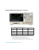
InfiniiVision 2000 X-Series Oscilloscopes—At a Glance Table 1 2000 X-Series Model Numbers, Bandwidths Bandwidth 70 MHz 100 MHz 200 MHz 2-Channel + 8 Logic Channels MSO MSO-X 2002A MSO-X 2012A MSO-X 2022A 4-Channel + 8 Logic Channels MSO MSO-X 2004A MSO-X 2014A MSO-X 2024A 2-Channel DSO DSO-X 2002A DSO-X 2012A DSO-X 2022A 4-Channel DSO DSO-X 2004A DSO-X 2014A DSO-X 2024A The Agilent InfiniiVision 2000 X- Series oscilloscopes deliver these features: • 70 MHz, 100 MHz, and 200 MHz bandwi
An MSO lets you debug your mixed- signal designs using analog signals and tightly correlated digital signals simultaneously. The 8 digital channels have a 1 GSa/s sample rate, with a 50 MHz toggle rate. • 8.5 inch WVGA display. • Interleaved 2 GSa/s or non- interleaved 1 GSa/s sample rate. • Interleaved 100 Kpts or non- interleaved 50 Kpts MegaZoom IV memory for the fastest waveform update rates, uncompromised. • All knobs are pushable for making quick selections.
In This Guide This guide shows how to use the InfiniiVision 2000 X- Series oscilloscopes.
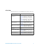
TIP Abbreviated instructions for pressing a series of keys and softkeys Instructions for pressing a series of keys are written in an abbreviated manner. Instructions for pressing [Key1], then pressing Softkey2, then pressing Softkey3 are abbreviated as follows: Press [Key1]> Softkey2 > Softkey3. The keys may be a front panel [Key] or a Softkey. Softkeys are the six keys located directly below the oscilloscope display.
Contents InfiniiVision 2000 X-Series Oscilloscopes—At a Glance In This Guide 1 3 5 Getting Started Inspect the Package Contents 19 Install the Optional LAN/VGA or GPIB Module Tilt the Oscilloscope for Easy Viewing Power-On the Oscilloscope 22 23 Connect Probes to the Oscilloscope 24 Maximum input voltage at analog inputs Do not float the oscilloscope chassis Input a Waveform 24 24 25 Recall the Default Oscilloscope Setup Use Auto Scale 22 25 26 Compensate Passive Probes 27 Learn the Fron
2 Horizontal Controls To adjust the horizontal (time/div) scale 44 To adjust the horizontal delay (position) 45 Panning and Zooming Single or Stopped Acquisitions 46 To change the horizontal time mode (Normal, XY, or Roll) XY Time Mode 48 To display the zoomed time base 47 50 To change the horizontal scale knob's coarse/fine adjustment setting 52 To position the time reference (left, center, right) Navigating the Time Base To navigate time 53 To navigate segments 3 52 53 53 Vertical Controls To
4 Math Waveforms To display math waveforms 63 To perform a transform function on an arithmetic operation To adjust the math waveform scale and offset Multiply 64 65 65 Add or Subtract 66 FFT Measurement 67 FFT Measurement Hints 71 FFT Units 72 FFT DC Value 72 FFT Aliasing 72 FFT Spectral Leakage 74 Units for Math Waveforms 5 74 Reference Waveforms To save a waveform to a reference waveform location To display a reference waveform 76 To scale and position reference waveforms To adjust reference
To display digital channels using AutoScale Interpreting the digital waveform display 83 84 To change the displayed size of the digital channels To switch a single channel on or off 86 To switch all digital channels on or off 86 To switch groups of channels on or off 86 To change the logic threshold for digital channels To reposition a digital channel 85 86 87 To display digital channels as a bus 88 Digital channel signal fidelity: Probe impedance and grounding 91 Input Impedance 92 Probe Grou
To define a new label 107 To load a list of labels from a text file you create To reset the label library to the factory default 9 108 109 Triggers Adjusting the Trigger Level Forcing a Trigger Edge Trigger 112 113 113 Pattern Trigger 116 Hex Bus Pattern Trigger Pulse Width Trigger 118 119 Video Trigger 121 To trigger on a specific line of video 125 To trigger on all sync pulses 126 To trigger on a specific field of the video signal 127 To trigger on all fields of the video signal 128 To trigger
11 Acquisition Control Running, Stopping, and Making Single Acquisitions (Run Control) 141 Overview of Sampling 143 Sampling Theory 143 Aliasing 143 Oscilloscope Bandwidth and Sample Rate Oscilloscope Rise Time 145 Oscilloscope Bandwidth Required 146 Memory Depth and Sample Rate 147 144 Selecting the Acquisition Mode 147 Normal Acquisition Mode 148 Peak Detect Acquisition Mode 148 Averaging Acquisition Mode 151 High Resolution Acquisition Mode 153 Acquiring to Segmented Memory 153 Navigating Segments 155
Peak-Peak 172 Maximum 172 Minimum 172 Amplitude 172 Top 173 Base 174 Overshoot 174 Preshoot 175 Average 176 DC RMS 176 AC RMS 177 Time Measurements 179 Period 179 Frequency 180 + Width 181 – Width 181 Burst Width 181 Duty Cycle 181 Rise Time 182 Fall Time 182 Delay 182 Phase 183 Measurement Thresholds 184 Measurement Window with Zoom Display 14 186 Mask Testing To create a mask from a "golden" waveform (Automask) Mask Test Setup Options Mask Statistics 187 189 192 To manually modify a mask file Agi
Building a Mask File 196 How is mask testing done? 15 198 Waveform Generator To select generated waveform types and settings To output the waveform generator sync pulse To specify the waveform generator output load To use waveform generator logic presets To restore waveform generator defaults 16 199 202 203 203 204 Save/Recall (Setups, Screens, Data) Saving Setups, Screen Images, or Data 205 To save setup files 207 To save BMP or PNG image files 207 To save CSV, ASCII XY, or BIN data files 208 To sav
17 Print (Screens) To print the oscilloscope's display 219 To set up network printer connections To specify the print options To specify the palette option 18 220 221 222 Utility Settings I/O Interface Settings 223 Setting up the Oscilloscope's LAN Connection 224 To establish a LAN connection 225 Stand-alone (Point-to-Point) Connection to a PC 226 File Explorer 227 Setting Oscilloscope Preferences 229 To choose "expand about" center or ground To disable/enable transparent backgrounds To load the d
To return the instrument 237 Configuring the [Quick Action] Key 19 238 Web Interface Accessing the Web Interface 242 Browser Web Control 243 Real Scope Remote Front Panel 244 Simple Remote Front Panel 245 Remote Programming via the Web Interface 246 Remote Programming with Agilent IO Libraries 247 Save/Recall 247 Saving Files via the Web Interface 247 Recalling Files via the Web Interface 249 Get Image 249 Identification Function 20 250 Instrument Utilities 251 Setting a Password 252 Referenc
Probes and Accessories 258 Passive Probes 258 Differential Probes 259 Current Probes 259 Accessories Available 260 Loading Licenses and Displaying License Information Licensed Options Available 261 Other Options Available 262 Upgrading to an MSO 262 Software and Firmware Updates 262 Binary Data (.
Agilent InfiniiVision 2000 X-Series Oscilloscopes User's Guide
Agilent InfiniiVision 2000 X-Series Oscilloscopes User's Guide 1 Getting Started Inspect the Package Contents 19 Tilt the Oscilloscope for Easy Viewing 22 Power-On the Oscilloscope 23 Connect Probes to the Oscilloscope 24 Input a Waveform 25 Recall the Default Oscilloscope Setup 25 Use Auto Scale 26 Compensate Passive Probes 27 Learn the Front Panel Controls and Connectors 28 Learn the Rear Panel Connectors 37 Learn the Oscilloscope Display 38 Access the Built-In Quick Help 40 This chapter describes the s
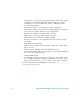
1 Getting Started • InfiniiVision 2000 X- Series oscilloscope. • Power cord (country of origin determines specific type). • Oscilloscope probes: • Two probes for 2- channel models. • Four probes for 4- channel models. • Documentation CD- ROM.
Getting Started 1 InfiniiVision 2000 X-Series oscilloscope N2862B probes (Qty 2 or 4) Documentation CD Digital Probe Kit* (MSO models only) Power cord (Based on country of origin) *N6459-60001 Digital Probe Kit contains: N6459-61601 8-channel cable (qyt 1) 01650-82103 2-inch probe ground leads (qyt 3) 5090-4832 Grabber (qty 10) Digital probe replacement parts are listed in the "Digital Channels" chapter.
1 Getting Started Install the Optional LAN/VGA or GPIB Module If you need to install a DSOXLAN LAN/VGA module or a DSOXGPIB GPIB module, perform this installation before you power on the oscilloscope. 1 If you need to remove a module before installing a different module, pinch the module's spring tabs, and gently remove the module from the slot. 2 To install a module, slide the module into the slot on the back until it is fully seated.
1 Getting Started Flip-Out Tabs Power-On the Oscilloscope Power Requirements Line voltage, frequency, and power: • ~Line 100- 120 Vac, 50/60/400 Hz • 100- 240 Vac, 50/60 Hz • 100 W max Ventilation Requirements The air intake and exhaust areas must be free from obstructions. Unrestricted air flow is required for proper cooling. Always ensure that the air intake and exhaust areas are free from obstructions.
1 Getting Started 2 The oscilloscope automatically adjusts for input line voltages in the range 100 to 240 VAC. The line cord provided is matched to the country of origin. WA R N I N G Always use a grounded power cord. Do not defeat the power cord ground. 3 Press the power switch. The power switch is located on the lower left corner of the front panel. The oscilloscope will perform a self- test and will be operational in a few seconds.
Getting Started WA R N I N G 1 Do not negate the protective action of the ground connection to the oscilloscope. The oscilloscope must remain grounded through its power cord. Defeating the ground creates an electric shock hazard. Input a Waveform The first signal to input to the oscilloscope is the Demo 2, Probe Comp signal. This signal is used for compensating probes. 1 Connect an oscilloscope probe from channel 1 to the Demo 2 (Probe Comp) terminal on the front panel.
1 Getting Started In the Save/Recall Menu, there are also options for restoring the complete factory settings (see “Recalling Default Setups" on page 216) or performing a secure erase (see “Performing a Secure Erase" on page 217). Use Auto Scale Use [Auto Scale] to automatically configure the oscilloscope to best display the input signals. 1 Press [Auto Scale].
1 Getting Started If you see the waveform, but the square wave is not shaped correctly as shown above, perform the procedure “Compensate Passive Probes" on page 27. If you do not see the waveform, make sure the probe is connected securely to the front panel channel input BNC and to the left side, Demo 2, Probe Comp terminal. How AutoScale Works Auto Scale analyzes any waveforms present at each channel and at the external trigger input. This includes the digital channels, if connected.
1 Getting Started If necessary, use a nonmetallic tool (supplied with the probe) to adjust the trimmer capacitor on the probe for the flattest pulse possible. On the N2862/63/90 probes, the trimmer capacitor is the yellow adjustment on the probe tip. On other probes, the trimmer capacitor is located on the probe BNC connector.
1 Getting Started 5. Tools keys 6. Trigger controls 7. Horizontal controls 8. Run Control keys 9. [Default Setup] key 10. [Auto Scale] key 11. Additional waveform controls 4. Entry knob 3. [Intensity] key 12. Measure controls 13. Waveform keys 2. Softkeys 14. File keys 1. Power switch 15. [Help] key 21. Waveform generator output 20. Digital channel inputs 19. USB Host port 18. Demo 2, Ground, 17. Analog 16 Vertical controls and Demo 1 channel terminals inputs 1.
1 Getting Started 4. Entry knob The Entry knob is used to select items from menus and to change values. The function of the Entry knob changes based upon the current menu and softkey selections. Note that the curved arrow symbol above the entry knob illuminates whenever the entry knob can be used to select a value. Also, note that when the Entry knob symbol appears on a softkey, you can use the Entry knob, to select values. Often, rotating the Entry knob is enough to make a selection.
Getting Started 7. Horizontal controls 1 The Horizontal controls consist of: • Horizontal scale knob — Turn the knob in the Horizontal section that is marked to adjust the time/div (sweep speed) setting. The symbols under the knob indicate that this control has the effect of spreading out or zooming in on the waveform using the horizontal scale. • Horizontal position knob — Turn the knob marked to pan through the waveform data horizontally.
1 32 Getting Started 10. [Auto Scale] key When you press the [AutoScale] key, the oscilloscope will quickly determine which channels have activity, and it will turn these channels on and scale them to display the input signals. See “Use Auto Scale" on page 26. 11. Additional waveform controls The additional waveform controls consist of: • [Math] key — provides access to math (add, subtract, etc.) waveform functions. See Chapter 4, “Math Waveforms,” starting on page 63.
1 Getting Started 12. Measure controls The measure controls consist of: • Cursors knob — Push this knob select cursors from a popup menu. Then, after the popup menu closes (either by timeout or by pushing the knob again), rotate the knob to adjust the selected cursor position. • [Cursors] key — Press this key to open a menu that lets you select the cursors mode and source. • [Meas] key — Press this key to access a set of predefined measurements. See Chapter 13, “Measurements,” starting on page 167. 13.
1 Getting Started 16. Vertical controls The Vertical controls consist of: • Analog channel on/off keys — Use these keys to switch a channel on or off, or to access a channel's menu in the softkeys. There is one channel on/off key for each analog channel. • Vertical scale knob — There are knobs marked for each channel. Use these knobs to change the vertical sensitivity (gain) of each analog channel. • Vertical position knobs — Use these knobs to change a channel's vertical position on the display.
Getting Started 19. USB Host port 1 This port is for connecting USB mass storage devices or printers to the oscilloscope. Connect a USB compliant mass storage device (flash drive, disk drive, etc.) to save or recall oscilloscope setup files and reference waveforms or to save data and screen images. See Chapter 16, “Save/Recall (Setups, Screens, Data),” starting on page 205. To print, connect a USB compliant printer.
1 Getting Started 3 Reinstall the front panel knobs. Front panel overlays may be ordered from "www.parts.agilent.
1 Getting Started Learn the Rear Panel Connectors For the following figure, refer to the numbered descriptions in the table that follows. 8. USB Device port 7. USB Host port 3. LAN/VGA option module 6. EXT TRIG IN connector 5. Calibration protect button 4. TRIG OUT connector L6GC>CCI6>C 9 :A:8IG>8 H=D8@ s &%%"&'%K! *%$+%$)%%=o s &%%"')%K! *%$+%=o &%% LViih B6M 3. GPIB option module 3. Module slot 2. Kensington lock hole 1. Power cord connector 1.
1 Getting Started 4. TRIG OUT connector Trigger output BNC connector. See “Setting the Rear Panel TRIG OUT Source" on page 232. 5. Calibration protect button See “To perform user calibration" on page 234. 6. EXT TRIG IN connector External trigger input BNC connector. See “External Trigger Input" on page 138 for an explanation of this feature. 8. USB Device port This port is for connecting the oscilloscope to a host PC.
1 Getting Started Analog channel sensitivity Trigger point, time reference Delay time Time/ div Run/Stop Trigger status type Trigger source Trigger level or digital threshold Status line Trigger level Information area Analog channels and ground levels Cursors defining measurement Digital channels Measurements Menu line Softkeys Figure 1 Interpreting the oscilloscope display Status line The top line of the display contains vertical, horizontal, and trigger setup information.
1 Getting Started Softkey labels These labels describe softkey functions. Typically, softkeys let you set up additional parameters for the selected mode or menu. Pressing the Back Back/Up key at the top of the menu hierarchy turns off softkey labels and displays additional status information describing channel offset and other configuration parameters. Access the Built-In Quick Help To view Quick Help 1 Press and hold the key or softkey for which you would like to view help.
1 Getting Started To select the user interface and Quick Help language To select the user interface and Quick Help language: 1 Press [Help], then press the Language softkey. 2 Repeatedly press and release the Language softkey or rotate the Entry knob until the desired language is selected. The following languages are available: English, French, German, Italian, Japanese, Korean, Portuguese, Russian, Simplified Chinese, Spanish, and Traditional Chinese.
1 42 Getting Started Agilent InfiniiVision 2000 X-Series Oscilloscopes User's Guide
Agilent InfiniiVision 2000 X-Series Oscilloscopes User's Guide 2 Horizontal Controls To adjust the horizontal (time/div) scale 44 To adjust the horizontal delay (position) 45 Panning and Zooming Single or Stopped Acquisitions 46 To change the horizontal time mode (Normal, XY, or Roll) 47 To display the zoomed time base 50 To change the horizontal scale knob's coarse/fine adjustment setting 52 To position the time reference (left, center, right) 52 Navigating the Time Base 53 The horizontal controls includ
2 Horizontal Controls Trigger point Time reference Delay time Time/ div Trigger source Trigger level or threshold Sample rate XY or Roll mode Normal time mode Figure 2 Zoomed time base Fine control Time reference Horizontal Menu The Horizontal Menu lets you select the time mode (Normal, XY, or Roll), enable Zoom, set the time base fine control (vernier), and specify the time reference. The current sample rate is displayed above the Fine and Time Ref softkeys.
2 Horizontal Controls Notice how the time/div information in the status line changes. The ∇ symbol at the top of the display indicates the time reference point. The horizontal scale knob works (in the Normal time mode) while acquisitions are running or when they are stopped. When running, adjusting the horizontal scale knob changes the sample rate. When stopped, adjusting the horizontal scale knob lets you zoom into acquired data. See "Panning and Zooming Single or Stopped Acquisitions" on page 46.
2 Horizontal Controls stopped, adjusting the horizontal scale knob lets you zoom into acquired data. See "Panning and Zooming Single or Stopped Acquisitions" on page 46. Note that the horizontal position knob has a different purpose in the Zoom display. See "To display the zoomed time base" on page 50. Panning and Zooming Single or Stopped Acquisitions When the oscilloscope is stopped, use the horizontal scale and position knobs to pan and zoom your waveform.
Horizontal Controls 2 To change the horizontal time mode (Normal, XY, or Roll) 1 Press [Horiz]. 2 In the Horizontal Menu, press Time Mode; then, select: • Normal — the normal viewing mode for the oscilloscope. In the Normal time mode, signal events occurring before the trigger are plotted to the left of the trigger point (▼) and signal events after the trigger plotted to the right of the trigger point. • XY — XY mode changes the display from a volts- versus- time display to a volts- versus- volts display.
2 Horizontal Controls XY Time Mode The XY time mode converts the oscilloscope from a volts- versus- time display to a volts- versus- volts display using two input channels. Channel 1 is the X- axis input, channel 2 is the Y- axis input. You can use various transducers so the display could show strain versus displacement, flow versus pressure, volts versus current, or voltage versus frequency.
2 Horizontal Controls 4 Press the [Cursors] key. 5 Set the Y2 cursor to the top of the signal, and set Y1 to the bottom of the signal. Note the ΔY value at the bottom of the display. In this example, we are using the Y cursors, but you could have used the X cursors instead. 6 Move the Y1 and Y2 cursors to the intersection of the signal and the Y axis. Again, note the ΔY value. Figure 4 Phase difference measurements, automatic and using cursors 7 Calculate the phase difference using the formula below.
2 Horizontal Controls NOTE Z-Axis Input in XY Display Mode (Blanking) When you select the XY display mode, the time base is turned off. Channel 1 is the X-axis input, channel 2 is the Y-axis input, and the rear panel EXT TRIG IN is the Z-axis input. If you only want to see portions of the Y versus X display, use the Z-axis input. Z-axis turns the trace on and off (analog oscilloscopes called this Z-axis blanking because it turned the beam on and off). When Z is low (<1.
2 Horizontal Controls These markers show the beginning and end of the Zoom window Time/div Time/div Delay time for zoomed for normal momentarily displays window window when the Horizontal position knob is turned Normal window Signal anomaly expanded in zoom window Zoom window Select Zoom The area of the normal display that is expanded is outlined with a box and the rest of the normal display is ghosted. The box shows the portion of the normal sweep that is expanded in the lower half.
2 Horizontal Controls Negative delay values indicate you're looking at a portion of the waveform before the trigger event, and positive values indicate you're looking at the waveform after the trigger event. To change the time/div of the normal window, turn off Zoom; then, turn the horizontal scale (sweep speed) knob. For information about using zoom mode for measurements, refer to "To isolate a pulse for Top measurement" on page 173 and "To isolate an event for frequency measurement" on page 180.
Horizontal Controls 2 The time reference position sets the initial position of the trigger event within acquisition memory and on the display, with delay set to 0. Turning the Horizontal scale (sweep speed) knob expands or contracts the waveform about the time reference point (∇). See "To adjust the horizontal (time/div) scale" on page 44. Turning the Horizontal position ( ) knob in Normal mode (not Zoom) moves the trigger point indicator (▼) to the left or right of the time reference point (∇).
2 Horizontal Controls 3 Press Play Mode; then, select: • Manual — to play through segments manually. In the Manual play mode: • Press the next segment. back and forward keys to go to the previous or • Press the softkey to go to the first segment. • Press the softkey to go to the last segment. • Auto — to play through segments in an automated fashion. In the Auto play mode: • Press the navigation keys to play backward, stop, or play forward in time.
Agilent InfiniiVision 2000 X-Series Oscilloscopes User's Guide 3 Vertical Controls To turn waveforms on or off (channel or math) 56 To adjust the vertical scale 57 To adjust the vertical position 57 To specify channel coupling 57 To specify bandwidth limiting 58 To change the vertical scale knob's coarse/fine adjustment setting 58 To invert a waveform 59 Setting Analog Channel Probe Options 59 The vertical controls include: • The vertical scale and position knobs for each analog channel.
3 Vertical Controls Channel, Volts/div Trigger source Trigger level or threshold Channel 1 ground level Channel 2 ground level The ground level of the signal for each displayed analog channel is identified by the position of the icon at the far- left side of the display. To turn waveforms on or off (channel or math) 1 Press an analog channel key turn the channel on or off (and to display the channel's menu). When a channel is on, its key is illuminated.
3 Vertical Controls To adjust the vertical scale 1 Turn the large knob above the channel key marked vertical scale (volts/division) for the channel. to set the The vertical scale knob changes the analog channel scale in a 1- 2- 5 step sequence (with a 1:1 probe attached) unless fine adjustment is enabled (see "To change the vertical scale knob's coarse/fine adjustment setting" on page 58). The analog channel Volts/Div value is displayed in the status line.
3 Vertical Controls TIP If the channel is DC coupled, you can quickly measure the DC component of the signal by simply noting its distance from the ground symbol. If the channel is AC coupled, the DC component of the signal is removed, allowing you to use greater sensitivity to display the AC component of the signal. 1 Press the desired channel key.
3 Vertical Controls When Fine adjustment is selected, you can change the channel's vertical sensitivity in smaller increments. The channel sensitivity remains fully calibrated when Fine is on. The vertical scale value is displayed in the status line at the top of the display. When Fine is turned off, turning the volts/division knob changes the channel sensitivity in a 1- 2- 5 step sequence. To invert a waveform 1 Press the desired channel key.
3 Vertical Controls The Probe Check softkey guides you through the process of compensating passive probes (such as the N2862A/B, N2863A/B, N2889A, N2890A, 10073C, 10074C, or 1165A probes). See Also • "To specify the channel units" on page 60 • "To specify the probe attenuation" on page 60 • "To specify the probe skew" on page 61 To specify the channel units 1 Press the probe's associated channel key. 2 In the Channel Menu, press Probe.
3 Vertical Controls If Amps is chosen as the units and a manual attenuation factor is chosen, then the units as well as the attenuation factor are displayed above the Probe softkey. To specify the probe skew When measuring time intervals in the nanoseconds (ns) range, small differences in cable length can affect the measurement. Use Skew to remove cable- delay errors between any two channels. 1 Probe the same point with both probes. 2 Press one of the probes associated channel key.
3 62 Vertical Controls Agilent InfiniiVision 2000 X-Series Oscilloscopes User's Guide
Agilent InfiniiVision 2000 X-Series Oscilloscopes User's Guide 4 Math Waveforms To display math waveforms 63 To perform a transform function on an arithmetic operation 64 To adjust the math waveform scale and offset 65 Add or Subtract 66 Multiply 65 FFT Measurement 67 Units for Math Waveforms 74 Math functions can be performed on analog channels. The resulting math waveform is displayed in light purple. You can use a math function on a channel even if you choose not to display the channel on- screen.
4 Math Waveforms 2 If f(t) is not already shown on the Function softkey, press the Function sofkey and select f(t): Displayed. 3 Use the Operator softkey to select an operator. For more information on the operators, see: • "Add or Subtract" on page 66 • "Multiply" on page 65 • "FFT Measurement" on page 67 4 Use the Source 1 softkey to select the analog channel on which to perform math. You can rotate the Entry knob or repetitively press the Source 1 softkey to make your selection.
4 Math Waveforms 2 Use the Operator, Source 1, and Source 2 softkeys to set up an arithmetic operation. 3 Press the Function softkey and select f(t): Displayed. 4 Use the Operator softkey to select a transform function (FFT). 5 Press the Source 1 softkey and select g(t) as the source. Note that g(t) is only available when you select a transform function in the previous step.
4 Math Waveforms Figure 5 See Also Example of Multiply Channel 1 by Channel 2 • "Units for Math Waveforms" on page 74 Add or Subtract When you select add or subtract, the Source 1 and Source 2 values are added or subtracted point by point, and the result is displayed. You can use subtract to make a differential measurement or to compare two waveforms. If your waveforms' DC offsets are larger than the dynamic range of the oscilloscope's input channels you will need to use a differential probe instead.
Math Waveforms Figure 6 See Also 4 Example of Subtract Channel 2 from Channel 1 • "Units for Math Waveforms" on page 74 FFT Measurement FFT is used to compute the fast Fourier transform using analog input channels or an arithmetic operation g(t). FFT takes the digitized time record of the specified source and transforms it to the frequency domain. When the FFT function is selected, the FFT spectrum is plotted on the oscilloscope display as magnitude in dBV versus frequency.
4 Math Waveforms • Source 1 — selects the source for the FFT. (See "To perform a transform function on an arithmetic operation" on page 64 for information about using g(t) as the source.) • Span — sets the overall width of the FFT spectrum that you see on the display (left to right). Divide span by 10 to calculate the number of Hertz per division. It is possible to set Span above the maximum available frequency, in which case the displayed spectrum will not take up the whole screen.
4 Math Waveforms • Rectangular — good frequency resolution and amplitude accuracy, but use only where there will be no leakage effects. Use on self- windowing waveforms such as pseudo- random noise, impulses, sine bursts, and decaying sinusoids. • Blackman Harris — window reduces time resolution compared to a rectangular window, but improves the capacity to detect smaller impulses due to lower secondary lobes. • Vertical Units — lets you select Decibels or V RMS as the units for the FFT vertical scale.
4 Math Waveforms You can make peak- to- peak, maximum, minimum, and average dB measurements on the FFT waveform. You can also find the frequency value at the first occurrence of the waveform maximum by using the X at Max Y measurement. The following FFT spectrum was obtained by connecting a 4 V, 75 kHz square wave to channel 1. Set the horizontal scale to 50 µs/div, vertical sensitivity to 1 V/div, Units/div to 20 dBV, Offset to - 60.
Math Waveforms 4 FFT Measurement Hints The number of points acquired for the FFT record can be up to 65,536, and when frequency span is at maximum, all points are displayed. Once the FFT spectrum is displayed, the frequency span and center frequency controls are used much like the controls of a spectrum analyzer to examine the frequency of interest in greater detail. Place the desired part of the waveform at the center of the screen and decrease frequency span to increase the display resolution.
4 Math Waveforms • Use the Hanning window. • Use Cursors to place an X cursor on the frequency of interest. • Adjust frequency span for better cursor placement. • Return to the Cursors Menu to fine tune the X cursor. For more information on the use of FFTs please refer to Agilent Application Note 243, The Fundamentals of Signal Analysis at "http://cp.literature.agilent.com/litweb/pdf/5952- 8898E.pdf".
Math Waveforms NOTE 4 Nyquist Frequency and Aliasing in the Frequency Domain The Nyquist frequency is the highest frequency that any real-time digitizing oscilloscope can acquire without aliasing. This frequency is half of the sample rate. Frequencies above the Nyquist frequency will be under sampled, which causes aliasing. The Nyquist frequency is also called the folding frequency because aliased frequency components fold back from that frequency when viewing the frequency domain.
4 Math Waveforms Because the frequency span goes from ≈ 0 to the Nyquist frequency, the best way to prevent aliasing is to make sure that the frequency span is greater than the frequencies of significant energy present in the input signal. FFT Spectral Leakage The FFT operation assumes that the time record repeats. Unless there is an integral number of cycles of the sampled waveform in the record, a discontinuity is created at the end of the record. This is referred to as leakage.
Agilent InfiniiVision 2000 X-Series Oscilloscopes User's Guide 5 Reference Waveforms To save a waveform to a reference waveform location 75 To display a reference waveform 76 To scale and position reference waveforms 77 To adjust reference waveform skew 77 To display reference waveform information 78 To save/recall reference waveform files to/from a USB storage device 78 Analog channel or math waveforms can be saved to one of two reference waveform locations in the oscilloscope.
5 Reference Waveforms 2 In the Reference Waveform Menu, press the Ref softkey and turn the Entry knob to select the desired reference waveform location. 3 Press the Source softkey and turn the Entry knob to select the source waveform. 4 Press the Save to R1/R2 softkey to save the waveform to the reference waveform location. NOTE To clear a reference waveform location Reference waveforms are non-volatile — they remain after power cycling or performing a default setup.
Reference Waveforms 5 One reference waveform can be displayed at a time. See Also • "To display reference waveform information" on page 78 To scale and position reference waveforms 1 Make sure the multiplexed scale and position knobs to the right of the [Ref] key are selected for the reference waveform. If the arrow to the left of the [Ref] key is not illuminated, press the key. 2 Turn the upper multiplexed knob to adjust the reference waveform scale.
5 Reference Waveforms 1 Display the desired reference waveform (see "To display a reference waveform" on page 76). 2 Press the Skew softkey and turn the Entry knob to adjust the reference waveform skew. To display reference waveform information 1 Press the [Ref] key to turn on reference waveforms. 2 In the Reference Waveform Menu, press the Options softkey.
Agilent InfiniiVision 2000 X-Series Oscilloscopes User's Guide 6 Digital Channels To connect the digital probes to the device under test 79 Acquiring waveforms using the digital channels 83 To display digital channels using AutoScale 83 Interpreting the digital waveform display 84 To switch all digital channels on or off 86 To switch groups of channels on or off 86 To switch a single channel on or off 86 To change the displayed size of the digital channels 85 To reposition a digital channel 87 To change th
6 Digital Channels Turning off power to the device under test would only prevent damage that might occur if you accidentally short two lines together while connecting probes. You can leave the oscilloscope powered on because no voltage appears at the probes. Off 2 Connect the digital probe cable to the DIGITAL Dn - D0 connector on the front panel of the mixed- signal oscilloscope. The digital probe cable is keyed so you can connect it only one way. You do not need to power- off the oscilloscope.
Digital Channels 6 Channel Pod Ground Circuit Ground 4 Connect a grabber to one of the probe leads. (Other probe leads are omitted from the figure for clarity.) Grabber 5 Connect the grabber to a node in the circuit you want to test.
6 Digital Channels 6 For high- speed signals, connect a ground lead to the probe lead, connect a grabber to the ground lead, and attach the grabber to ground in the device under test. Signal Ground Grabber 7 Repeat these steps until you have connected all points of interest.
6 Digital Channels Acquiring waveforms using the digital channels When you press [Run/Stop] or [Single] to run the oscilloscope, the oscilloscope examines the input voltage at each input probe. When the trigger conditions are met the oscilloscope triggers and displays the acquisition. For digital channels, each time the oscilloscope takes a sample it compares the input voltage to the logic threshold.
6 Digital Channels Any digital channel with an active signal will be displayed. Any digital channels without active signals will be turned off. • To undo the effects of AutoScale, press the Undo AutoScale softkey before pressing any other key. This is useful if you have unintentionally pressed the [AutoScale] key or do not like the settings AutoScale has selected. This will return the oscilloscope to its previous settings. See also: "How AutoScale Works" on page 27.
6 Digital Channels Delay time Time/ div Trigger mode or run status Trigger type and source Threshold level Activity indicators Digital channel identifiers Waveform size Activity indicator Turn individual channels on/off Turn groups of channels on/off Threshold menu key When any digital channels are turned on, an activity indicator is displayed in the status line at the bottom of the display. A digital channel can be always high ( ), always low ( ), or actively toggling logic states ( ).
6 Digital Channels The sizing control lets you spread out or compress the digital traces vertically on the display for more convenient viewing. To switch a single channel on or off 1 With the Digital Channel Menu displayed, rotate the Entry knob to select the desired channel from the popup menu. 2 Push the Entry knob or press the softkey that is directly below the popup menu to switch the selected channel on or off.
Digital Channels 6 3 Press the D7 - D0 softkey, then select a logic family preset or select User to define your own threshold. Logic family Threshold Voltage TTL +1.4 V CMOS +2.5 V ECL –1.3 V User Variable from –8 V to +8 V The threshold you set applies to all channels within the selected D7 - D0 group. Each of the two channel groups can be set to a different threshold if desired. Values greater than the set threshold are high (1) and values less than the set threshold are low (0).
6 Digital Channels To display digital channels as a bus Digital channels may be grouped and displayed as a bus, with each bus value displayed at the bottom of the display in hex or binary. You can create up to two buses. To configure and display each bus, press the [Digital] key on the front panel. Then press the Bus softkey. Next, select a bus. Rotate the Entry knob, then press the Entry knob or the Bus1/Bus2 softkey to switch it on.
Digital Channels 6 Bus values can be shown in hex or binary. Using cursors to read bus values To read the digital bus value at any point using the cursors: 1 Turn on Cursors (by pressing the [Cursors] key on the front panel) 2 Press the cursor Mode softkey and change the mode to Hex or Binary. 3 Press the Source softkey and select Bus1 or Bus2. 4 Use the Entry knob and the X1 and X2 softkeys to position the cursors where you want to read the bus values.
6 Digital Channels X1 cursor X2 cursor Bus values Set cursors mode to Binary or Hex Select Bus1 or Bus2 source Bus values at cursors shown here When you press the [Digital] key to display the Digital Channel Menu, the digital activity indicator is shown where the cursor values were and the bus values at the cursors are displayed in the graticule. Bus values are displayed when using Pattern trigger The bus values are also displayed when using the Pattern trigger function.
Digital Channels Trigger pattern definition Bus values displayed Analog channel values at cursor 6 Digital channel values at cursor See "Pattern Trigger" on page 116 for more information on Pattern triggering. Digital channel signal fidelity: Probe impedance and grounding When using the mixed- signal oscilloscope you may encounter problems that are related to probing. These problems fall into two categories: probe loading and probe grounding.
6 Digital Channels Input Impedance The logic probes are passive probes, which offer high input impedance and high bandwidths. They usually provide some attenuation of the signal to the oscilloscope, typically 20 dB. Passive probe input impedance is generally specified in terms of a parallel capacitance and resistance. The resistance is the sum of the tip resistor value and the input resistance of the test instrument (see the following figure).
Digital Channels Figure 10 6 High-Frequency Probe Equivalent Circuit The impedance plots for the two models are shown in these figures. By comparing the two plots, you can see that both the series tip resistor and the cable's characteristic impedance extend the input impedance significantly. The stray tip capacitance, which is generally small (1 pF), sets the final break point on the impedance chart.
6 Digital Channels 100 k High Frequency Model Impedance 10 k 1k Typical Model 100 10 1 10 kHz 100 kHz 1 MHz 10 MHz 100 MHz 1 GHz Frequency Figure 11 Impedance versus Frequency for Both Probe Circuit Models The logic probes are represented by the high- frequency circuit model shown above. They are designed to provide as much series tip resistance as possible. Stray tip capacitance to ground is minimized by the proper mechanical design of the probe tip assembly.
Digital Channels 6 Increasing the ground inductance (L), increasing the current (di) or decreasing the transition time (dt), will all result in increasing the voltage (V). When this voltage exceeds the threshold voltage defined in the oscilloscope, a false data measurement will occur. Sharing one probe ground with many probes forces all the current that flows into each probe to return through the same common ground inductance of the probe whose ground return is used.
6 Digital Channels you will discover the problem through random glitches or inconsistent data measurements. Use the analog channels to view ringing and perturbations. Best Probing Practices Because of the variables L, di, and dt, you may be unsure how much margin is available in your measurement setup.
6 Digital Channels Table 3 Digital Probe Replacement Parts Part Number Description N6459-60001 Digital probe kit, contains: N6459-61601 8-channel cable, 01650-82103 2-inch probe grounds (qty 3), and 5090-4832 grabbers (qty 10) N6459-61601 8-channel cable with 8 probe leads and 1 pod ground lead (qty 1) 5959-9333 Replacement probe leads (qty 5), also contains 01650-94309 probe labels 5959-9334 Replacement 2-inch probe grounds (qty 5) 5959-9335 Replacement pod ground leads (qty 5) 5090-4833 G
6 98 Digital Channels Agilent InfiniiVision 2000 X-Series Oscilloscopes User's Guide
Agilent InfiniiVision 2000 X-Series Oscilloscopes User's Guide 7 Display Settings To adjust waveform intensity 99 To set or clear persistence 101 To clear the display 102 To select the grid type 102 To adjust the grid intensity 103 To freeze the display 103 To adjust waveform intensity You can adjust the intensity of displayed waveforms to account for various signal characteristics, such as fast time/div settings and low trigger rates.
7 100 Display Settings Figure 13 Amplitude Modulation Shown at 100% Intensity Figure 14 Amplitude Modulation Shown at 40% Intensity Agilent InfiniiVision 2000 X-Series Oscilloscopes User's Guide
7 Display Settings To set or clear persistence With persistence, the oscilloscope updates the display with new acquisitions, but does not immediately erase the results of previous acquisitions. All previous acquisitions are displayed with reduced intensity. New acquisitions are shown in their normal color with normal intensity. Waveform persistence is kept only for the current display area; you cannot pan and zoom the persistence display. To use persistence: 1 Press the [Display] key.
7 Display Settings 3 To erase the results of previous acquisitions from the display, press the Clear Persistence softkey. The oscilloscope will start to accumulate acquisitions again. 4 To return the oscilloscope to the normal display mode, turn off persistence; then, press the Clear Persistence softkey. Turning off persistence does not clear the display. The display is cleared if you press the Clear Display softkey or if you press the [AutoScale] key (which also turns off persistence).
7 Display Settings 1 Press [Display]. 2 Press the Grid softkey; then, turn the Entry knob type. to select the grid To adjust the grid intensity To adjust the display grid (graticule) intensity: 1 Press [Display]. 2 Press the Intensity softkey; then, turn the Entry knob intensity of the displayed grid. to change the The intensity level is shown in the Intensity softkey and is adjustable from 0 to 100%.
7 104 Display Settings Agilent InfiniiVision 2000 X-Series Oscilloscopes User's Guide
Agilent InfiniiVision 2000 X-Series Oscilloscopes User's Guide 8 Labels To turn the label display on or off 105 To assign a predefined label to a channel 106 To define a new label 107 To load a list of labels from a text file you create 108 To reset the label library to the factory default 109 You can define labels and assign them to each analog input channel, or you can turn labels off to increase the waveform display area. Labels can also be applied to digital channels on MSO models.
8 Labels 2 To turn the labels off, press the [Label] key again. To assign a predefined label to a channel 1 Press the [Label] key. 2 Press the Channel softkey, then turn the Entry knob or successively press the Channel softkey to select a channel for label assignment.
Labels 8 The figure above shows the list of channels and their default labels. The channel does not have to be turned on to have a label assigned to it. 3 Press the Library softkey, then turn the Entry knob or successively press the Library softkey to select a predefined label from the library. 4 Press the Apply New Label softkey to assign the label to your selected channel. 5 Repeat the above procedure for each predefined label you want to assign to a channel.
8 Labels Turning the Entry knob selects a character to enter into the highlighted position shown in the "New label =" line above the softkeys and in the Spell softkey. Labels can be up to ten characters in length. 4 Press the Enter softkey to enter the selected character and to go to the next character position. 5 You may position the highlight on any character in the label name by successively pressing the Enter softkey.
8 Labels 3 Load the list into the oscilloscope using the File Explorer (press [Utility] > File Explorer). NOTE Label List Management When you press the Library softkey, you will see a list of the last 75 labels used. The list does not save duplicate labels. Labels can end in any number of trailing digits. As long as the base string is the same as an existing label in the library, the new label will not be put in the library.
8 110 Labels Agilent InfiniiVision 2000 X-Series Oscilloscopes User's Guide
Agilent InfiniiVision 2000 X-Series Oscilloscopes User's Guide 9 Triggers Adjusting the Trigger Level 112 Forcing a Trigger 113 Edge Trigger 113 Pattern Trigger 116 Pulse Width Trigger 119 Video Trigger 121 A trigger setup tells the oscilloscope when to acquire and display data. For example, you can set up to trigger on the rising edge of the analog channel 1 input signal. You can adjust the vertical level used for analog channel edge detection by turning the Trigger Level knob.
9 Triggers You can save trigger setups along with the oscilloscope setup (see Chapter 16, “Save/Recall (Setups, Screens, Data),” starting on page 205). Triggers - General Information A triggered waveform is one in which the oscilloscope begins tracing (displaying) the waveform, from the left side of the display to the right, each time a particular trigger condition is met.
9 Triggers The trigger level for a selected digital channel is set using the threshold menu in the Digital Channel Menu. Press the [Digital] key on the front panel, then press the Thresholds softkey to set the threshold level (TTL, CMOS, ECL, or user defined) for the selected digital channel group. The threshold value is displayed in the upper- right corner of the display. The line trigger level is not adjustable. This trigger is synchronized with the power line supplied to the oscilloscope.
9 Triggers • Analog channel, 1 to the number of channels • Digital channel (on mixed- signal oscilloscopes), D0 to the number of digital channels minus one. • External. • Line. • WaveGen (not available when the DC or Noise waveforms are selected). You can choose a channel that is turned off (not displayed) as the source for the edge trigger. The selected trigger source is indicated in the upper- right corner of the display next to the slope symbol: • 1 through 4 = analog channels.
9 Triggers NOTE Alternating edge mode is useful when you want to trigger on both edges of a clock (for example, DDR signals). Either edge mode is useful when you want to trigger on any activity of a selected source. All modes operate up to the bandwidth of the oscilloscope except Either edge mode, which has a limitation. Either edge mode will trigger on Constant Wave signals up to 100 MHz, but can trigger on isolated pulses down to 1/(2*oscilloscope's bandwidth).
9 Triggers Pattern Trigger The Pattern trigger identifies a trigger condition by looking for a specified pattern. This pattern is a logical AND combination of the channels. Each channel can have a value of 0 (low), 1 (high), or don't care (X). A rising or falling edge can be specified for one channel included in the pattern. You can also trigger on a hex bus value as described on "Hex Bus Pattern Trigger" on page 118. 1 Press the [Trigger] key.
9 Triggers • 0 sets the pattern to zero (low) on the selected channel. A low is a voltage level that is less than the channel's trigger level or threshold level. • 1 sets the pattern to 1 (high) on the selected channel. A high is a voltage level that is greater than the channel's trigger level or threshold level. • X sets the pattern to don't care on the selected channel. Any channel set to don't care is ignored and is not used as part of the pattern.
9 Triggers NOTE Specifying an Edge in a Pattern You are allowed to specify only one rising or falling edge term in the pattern. If you define an edge term, then select a different channel in the pattern and define another edge term, the previous edge definition is changed to a don't care. Hex Bus Pattern Trigger You can specify a bus value on which to trigger. To do this, first define the bus. See "To display digital channels as a bus" on page 88 for details.
Triggers 9 Pulse Width Trigger Pulse Width (glitch) triggering sets the oscilloscope to trigger on a positive or negative pulse of a specified width. If you want to trigger on a specific timeout value, use Pattern trigger in the Trigger Menu (see "Pattern Trigger" on page 116). 1 Press the [Trigger] key. 2 In the Trigger Menu, press the Trigger softkey; then, turn the Entry knob to select Pulse Width. 3 Press the Source softkey; then, rotate the Entry knob to select a channel source for the trigger.
9 Triggers • For digital channels, press the [Digital] key and select Thresholds to set the threshold level. The value of the trigger level or digital threshold is displayed in the upper- right corner of the display. 5 Press the pulse polarity softkey to select positive ( polarity for the pulse width you want to capture. ) or negative ( ) The selected pulse polarity is displayed in the upper- right corner of the display.
Triggers 10 ns 15 ns 12 ns 9 Trigger 7 Select the qualifier time set softkey (< or >), then rotate the Entry knob to set the pulse width qualifier time. The qualifiers can be set as follows: • 2 ns to 10 s for > or < qualifier (5 ns to 10 s for 350 MHz bandwidth models). • 10 ns to 10 s for >< qualifier, with minimum difference of 5 ns between upper and lower settings.
9 Triggers NOTE It is important, when using a 10:1 passive probe, that the probe is correctly compensated. The oscilloscope is sensitive to this and will not trigger if the probe is not properly compensated, especially for progressive formats. 1 Press the [Trigger] key. 2 In the Trigger Menu, press the Trigger softkey; then, turn the Entry knob to select Video. 3 Press the Source softkey and select any analog channel as the video trigger source.
9 Triggers NOTE Provide Correct Matching Many video signals are produced from 75 Ω sources. To provide correct matching to these sources, a 75 Ω terminator (such as an Agilent 11094B) should be connected to the oscilloscope input. 4 Press the sync polarity softkey to set the Video trigger to either positive ( ) or negative ( ) sync polarity. 5 Press the Settings softkey. 6 In the Video Trigger Menu, press the Standard softkey to set the video standard.
9 Triggers • Horizontal time/division is set to 10 µs/div for NTSC/PAL/SECAM standards. • Horizontal delay is set so that trigger is at first horizontal division from the left. You can also press [Analyze]> Features and then select Video to quickly access the video triggering automatic set up and display options. 8 Press the Mode softkey to select the portion of the video signal that you would like to trigger on.
9 Triggers • "To trigger on all sync pulses" on page 126 • "To trigger on a specific field of the video signal" on page 127 • "To trigger on all fields of the video signal" on page 128 • "To trigger on odd or even fields" on page 129 To trigger on a specific line of video Video triggering requires greater than 1/2 division of sync amplitude with any analog channel as the trigger source.
9 Triggers Figure 15 Example: Triggering on Line 136 To trigger on all sync pulses To quickly find maximum video levels, you could trigger on all sync pulses. When All Lines is selected as the Video trigger mode, the oscilloscope will trigger on all horizontal sync pulses. 1 Press the [Trigger] key. 2 In the Trigger Menu, press the Trigger softkey; then, turn the Entry knob to select Video. 3 Press the Settings softkey, then press the Standard softkey to select the appropriate TV standard.
9 Triggers Figure 16 Triggering on All Lines To trigger on a specific field of the video signal To examine the components of a video signal, trigger on either Field 1 or Field 2 (available for interleaved standards). When a specific field is selected, the oscilloscope triggers on the rising edge of the first serration pulse in the vertical sync interval in the specified field (1 or 2). 1 Press the [Trigger] key. 2 In the Trigger Menu, press the Trigger softkey; then, turn the Entry knob to select Video.
9 Triggers Figure 17 Triggering on Field 1 To trigger on all fields of the video signal To quickly and easily view transitions between fields, or to find the amplitude differences between the fields, use the All Fields trigger mode. 1 Press the [Trigger] key. 2 In the Trigger Menu, press the Trigger softkey; then, turn the Entry knob to select Video. 3 Press the Settings softkey, then press the Standard softkey to select the appropriate TV standard. 4 Press the Mode softkey and select All Fields.
9 Triggers Figure 18 Triggering on All Fields To trigger on odd or even fields To check the envelope of your video signals, or to measure worst case distortion, trigger on the odd or even fields. When Field 1 is selected, the oscilloscope triggers on color fields 1 or 3. When Field 2 is selected, the oscilloscope triggers on color fields 2 or 4. 1 Press the [Trigger] key. 2 In the Trigger Menu, press the Trigger softkey; then, turn the Entry knob to select Video.
9 Triggers starts on Line 4. In the case of NTSC video, the oscilloscope will trigger on color field 1 alternating with color field 3 (see the following figure). This setup can be used to measure the envelope of the reference burst. Figure 19 Triggering on Color Field 1 Alternating with Color Field 3 If a more detailed analysis is required, then only one color field should be selected to be the trigger. You can do this by using the Field Holdoff softkey in the Video Trigger Menu.
Triggers Table 4 Half-field holdoff time Standard Time NTSC 8.
9 132 Triggers Agilent InfiniiVision 2000 X-Series Oscilloscopes User's Guide
Agilent InfiniiVision 2000 X-Series Oscilloscopes User's Guide 10 Trigger Mode/Coupling To select the Auto or Normal trigger mode 134 To select the trigger coupling 136 To enable or disable trigger noise rejection 137 To enable or disable trigger HF Reject 137 To set the trigger holdoff 138 External Trigger Input 138 To access the Trigger Mode and Coupling Menu: • In the Trigger section of the front panel, press the [Mode/Coupling] key.
10 Trigger Mode/Coupling To select the Auto or Normal trigger mode When the oscilloscope is running, the trigger mode tells the oscilloscope what to do when triggers are not occurring. In the Auto trigger mode (the default setting), if the specified trigger conditions are not found, triggers are forced and acquisitions are made so that signal activity is displayed on the oscilloscope. In the Normal trigger mode, triggers and acquisitions only occur when the specified trigger conditions are found.
10 Trigger Mode/Coupling Trigger Indicator The trigger indicator at the top right of the display shows whether triggers are occurring. In the Auto trigger mode, the trigger indicator can show: • Auto? (flashing) — the trigger condition is not found (after the pre- trigger buffer has filled), and forced triggers and acquisitions are occurring. • Auto (not flashing) — the trigger condition is found (or the pre- trigger buffer is being filled).
10 Trigger Mode/Coupling • "To position the time reference (left, center, right)" on page 52 To select the trigger coupling 1 Press the [Mode/Coupling] key. 2 In the Trigger Mode and Coupling Menu, press the Coupling softkey; then, turn the Entry knob to select: • DC coupling — allows DC and AC signals into the trigger path. • AC coupling — places a 10 Hz high- pass filter in the trigger path removing any DC offset voltage from the trigger waveform.
10 Trigger Mode/Coupling Note that Trigger Coupling is independent of Channel Coupling (see "To specify channel coupling" on page 57). To enable or disable trigger noise rejection Noise Rej adds additional hysteresis to the trigger circuitry. By increasing the trigger hysteresis band, you reduce the possibility of triggering on noise. However, this also decreases the trigger sensitivity so that a slightly larger signal is required to trigger the oscilloscope. 1 Press the [Mode/Coupling] key.
10 Trigger Mode/Coupling To set the trigger holdoff Trigger holdoff sets the amount of time the oscilloscope waits after a trigger before re- arming the trigger circuitry. Use the holdoff to trigger on repetitive waveforms that have multiple edges (or other events) between waveform repetitions. You can also use holdoff to trigger on the first edge of a burst when you know the minimum time between bursts.
Trigger Mode/Coupling CAUTION 10 Maximum voltage at oscilloscope external trigger input CAT I 300 Vrms, 400 Vpk; transient overvoltage 1.6 kVpk 1 M ohm input: For steady-state sinusoidal waveforms derate at 20 dB/decade above 57 kHz to a minimum of 5 Vpk With N2863A 10:1 probe: CAT I 600 V, CAT II 300 V (DC + peak AC) With 10073C or 10074C 10:1 probe: CAT I 500 Vpk, CAT II 400 Vpk The external trigger input impedance is 1M Ohm. This lets you use passive probes for general- purpose measurements.
10 Trigger Mode/Coupling 140 Agilent InfiniiVision 2000 X-Series Oscilloscopes User's Guide
Agilent InfiniiVision 2000 X-Series Oscilloscopes User's Guide 11 Acquisition Control Running, Stopping, and Making Single Acquisitions (Run Control) 141 Overview of Sampling 143 Selecting the Acquisition Mode 147 Acquiring to Segmented Memory 153 This chapter shows how to use the oscilloscope's acquisition and run controls.
11 Acquisition Control When you press [Single], the display is cleared, the trigger mode is temporarily set to Normal (to keep the oscilloscope from auto- triggering immediately), the trigger circuitry is armed, the [Single] key is illuminated, and the oscilloscope waits until a trigger condition occurs before it displays a waveform. When the oscilloscope triggers, the single acquisition is displayed and the oscilloscope is stopped (the [Run/Stop] key is illuminated in red).
Acquisition Control 11 Overview of Sampling To understand the oscilloscope's sampling and acquisition modes, it is helpful to understand sampling theory, aliasing, oscilloscope bandwidth and sample rate, oscilloscope rise time, oscilloscope bandwidth required, and how memory depth affects sample rate.
11 Acquisition Control Oscilloscope Bandwidth and Sample Rate An oscilloscope's bandwidth is typically described as the lowest frequency at which input signal sine waves are attenuated by 3 dB (- 30% amplitude error). At the oscilloscope bandwidth, sampling theory says the required sample rate is fS = 2fBW. However, the theory assumes there are no frequency components above fMAX (fBW in this case) and it requires a system with an ideal brick- wall frequency response.
Acquisition Control 11 %Y7 6iiZcjVi^dc "(Y7 6a^VhZY [gZfjZcXn XdbedcZcih [H$) [C [H ;gZfjZcXn Limiting oscilloscope bandwidth (fBW) to 1/4 the sample rate (fS/4) reduces frequency components above the Nyquist frequency (fN). Figure 23 Sample Rate and Oscilloscope Bandwidth So, in practice, an oscilloscope's sample rate should be four or more times its bandwidth: fS = 4fBW. This way, there is less aliasing, and aliased frequency components have a greater amount of attenuation.
11 Acquisition Control Oscilloscope Bandwidth Required The oscilloscope bandwidth required to accurately measure a signal is primarily determined by the signal's rise time, not the signal's frequency. You can use these steps to calculate the oscilloscope bandwidth required: 1 Determine the fastest edge speeds. You can usually obtain rise time information from published specifications for devices used in your designs. 2 Compute the maximum "practical" frequency component. From Dr. Howard W.
11 Acquisition Control Memory Depth and Sample Rate The number of points of oscilloscope memory is fixed, and there is a maximum sample rate associated with oscilloscope's analog- to- digital converter; however, the actual sample rate is determined by the time of the acquisition (which is set according to the oscilloscope's horizontal time/div scale). sample rate = number of samples / time of acquisition For example, when storing 50 µs of data in 50,000 points of memory, the actual sample rate is 1 GSa/s.
11 Acquisition Control • Normal — at slower time/div settings, normal decimation occurs, and there is no averaging. Use this mode for most waveforms. See "Normal Acquisition Mode" on page 148. • Peak Detect — at slower time/div settings, the maximum and minimum samples in the effective sample period are stored. Use this mode for displaying narrow pulses that occur infrequently. See "Peak Detect Acquisition Mode" on page 148.
Acquisition Control 11 Glitch or Narrow Pulse Capture A glitch is a rapid change in the waveform that is usually narrow as compared to the waveform. Peak detect mode can be used to more easily view glitches or narrow pulses. In peak detect mode, narrow glitches and sharp edges are displayed more brightly than when in Normal acquire mode, making them easier to see. To characterize the glitch, use the cursors or the automatic measurement capabilities of the oscilloscope.
11 Acquisition Control Figure 25 Sine With Glitch, Peak Detect Mode Using Peak Detect Mode to Find a Glitch 1 Connect a signal to the oscilloscope and obtain a stable display. 2 To find the glitch, press the [Acquire] key; then, press the Acq Mode softkey until Peak Detect is selected. 3 Press the [Display] key then press the ∞ Persistence (infinite persistence) softkey. Infinite persistence updates the display with new acquisitions but does not erase previous acquisitions.
11 Acquisition Control Use the horizontal position knob ( ) to pan through the waveform to set the expanded portion of the normal window around the glitch. Averaging Acquisition Mode The Averaging mode lets you average multiple acquisitions together to reduce noise and increase vertical resolution (at all time/div settings). Averaging requires a stable trigger. The number of averages can be set from 2 to 65536 in power- of- 2 increments.
11 Acquisition Control 152 Figure 26 Random noise on the displayed waveform Figure 27 128 Averages used to reduce random noise Agilent InfiniiVision 2000 X-Series Oscilloscopes User's Guide
11 Acquisition Control See Also • Chapter 10, “Trigger Mode/Coupling,” starting on page 133 High Resolution Acquisition Mode In High Resolution mode, at slower time/div settings when decimation would normally occur, extra samples are averaged in order to reduce random noise, produce a smoother trace on the screen, and effectively increase vertical resolution. High Resolution mode averages sequential sample points within the same acquisition.
11 Acquisition Control When capturing multiple infrequent trigger events it is advantageous to divide the oscilloscope's memory into segments. This lets you capture signal activity without capturing long periods of signal inactivity. Each segment is complete with all analog channel and digital channel (on MSO models) data. When using segmented memory, use the Analyze Segments feature (see "Infinite Persistence with Segmented Memory" on page 155) to show infinite persistence across all acquired segments.
Acquisition Control 11 Progress indicator Sample rate See Also • "Navigating Segments" on page 155 • "Infinite Persistence with Segmented Memory" on page 155 • "Segmented Memory Re- Arm Time" on page 156 • "Saving Data from Segmented Memory" on page 156 Navigating Segments 1 Press the Current Seg softkey and turn the Entry knob to display the desired segment along with a time tag indicating the time from the first trigger event. You can also navigate segments using the [Navigate] key and controls.
11 Acquisition Control Segmented Memory Re-Arm Time After each segment fills, the oscilloscope re- arms and is ready to trigger in about 8 µs. Remember though, for example: if the horizontal time per division control is set to 5 µs/div, and the Time Reference is set to Center, it will take at least 50 µs to fill all ten divisions and re- arm. (That is 25 µs to capture pre- trigger data and 25 µs to capture post- trigger data.
Agilent InfiniiVision 2000 X-Series Oscilloscopes User's Guide 12 Cursors To make cursor measurements 158 Cursor Examples 161 Cursors are horizontal and vertical markers that indicate X- axis values and Y- axis values on a selected waveform source. You can use cursors to make custom voltage, time, phase, or ratio measurements on oscilloscope signals. Cursor information is displayed in the right- side information area. Cursors are not always limited to the visible display.
12 Cursors Y Cursors Y cursors are horizontal dashed lines that adjust vertically and can be used to measure Volts or Amps, dependent on the channel Probe Units setting, or they can measure ratios (%). When math functions are used as a source, the measurement units correspond to that math function. The Y1 cursor is the short- dashed horizontal line and the Y2 cursor is the long- dashed horizontal line.
12 Cursors • Track Waveform — As you move a marker horizontally, the vertical amplitude of the waveform is tracked and measured. The time and voltage positions are shown for the markers. The vertical (Y) and horizontal (X) differences between the markers are shown as ΔX and ΔY values. • Binary — Logic levels of displayed waveforms at the current X1 and X2 cursor positions are displayed above the softkeys in binary. The display is color coded to match the color of the related channel's waveform.
12 Cursors • Press the Cursors softkey; then, turn the Entry knob. The X1 X2 linked and Y1 Y2 linked selections let you adjust both cursors at the same time, while the delta value remains the same. This can be useful, for example, for checking pulse width variations in a pulse train. The currently selected cursor(s) display brighter than the other cursors. 6 To change the cursor units, press the Units softkey. In the Cursor Units Menu: You can press the X Units softkey to select: • Seconds (s).
Cursors 12 Cursor Examples Figure 28 Cursors used to measure pulse widths other than middle threshold points Agilent InfiniiVision 2000 X-Series Oscilloscopes User's Guide 161
12 Cursors Figure 29 Cursors measure frequency of pulse ringing Expand the display with Zoom mode, then characterize the event of interest with the cursors.
Cursors Figure 30 12 Cursors track Zoom window Put the X1 cursor on one side of a pulse and the X2 cursor on the other side of the pulse.
12 Cursors Figure 31 Measuring pulse width with cursors Press the X1 X2 linked softkey and move the cursors together to check for pulse width variations in a pulse train.
Cursors Figure 32 12 Moving the cursors together to check pulse width variations Agilent InfiniiVision 2000 X-Series Oscilloscopes User's Guide 165
12 Cursors 166 Agilent InfiniiVision 2000 X-Series Oscilloscopes User's Guide
Agilent InfiniiVision 2000 X-Series Oscilloscopes User's Guide 13 Measurements To make automatic measurements 168 Measurements Summary 169 Voltage Measurements 171 Time Measurements 179 Measurement Thresholds 184 Measurement Window with Zoom Display 186 The [Meas] key lets you make automatic measurements on waveforms. Some measurements can only be made on analog input channels.
13 Measurements To make automatic measurements 1 Press the [Meas] key to display the Measurement Menu. 2 Press the Source softkey to select the channel, running math function, or reference waveform to be measured. Only channels, math functions, or reference waveforms that are displayed are available for measurements.
Measurements 13 For more information on the types of measurements, see "Measurements Summary" on page 169. 4 The Settings softkey will be available to make additional measurement settings on some measurements. 5 Press the Add Measurement softkey or push the Entry knob to display the measurement. 6 To turn off measurements, press the [Meas] key again. Measurements are erased from the display.
13 Measurements Measurement Valid for Math FFT* Valid for Digital Channels Notes "Base" on page 174 "Burst Width" on page 181 "Delay" on page 182 Measures between two sources. Press Settings to specify the second source. "Duty Cycle" on page 181 Yes "Fall Time" on page 182 "Frequency" on page 180 Yes "Maximum" on page 172 Yes "Minimum" on page 172 Yes "Overshoot" on page 174 "Peak-Peak" on page 172 "Period" on page 179 Yes Yes "Phase" on page 183 Measures between two sources.
Measurements 13 Snapshot All The Snapshot All measurement type displays a popup containing a snapshot of all the single waveform measurements. You can also configure the [Quick Action] key to display the Snapshot All popup. See "Configuring the [Quick Action] Key" on page 238. Voltage Measurements The following figure shows the voltage measurement points.
13 Measurements The units of math waveforms are described in "Units for Math Waveforms" on page 74. • "Peak- Peak" on page 172 • "Maximum" on page 172 • "Minimum" on page 172 • "Amplitude" on page 172 • "Top" on page 173 • "Base" on page 174 • "Overshoot" on page 174 • "Preshoot" on page 175 • "Average" on page 176 • "DC RMS" on page 176 • "AC RMS" on page 177 Peak-Peak The peak- to- peak value is the difference between Maximum and Minimum values. The Y cursors show the values being measured.
13 Measurements Top The Top of a waveform is the mode (most common value) of the upper part of the waveform, or if the mode is not well defined, the top is the same as Maximum. The Y cursor shows the value being measured. See Also • "To isolate a pulse for Top measurement" on page 173 To isolate a pulse for Top measurement The following figure shows how to use Zoom mode to isolate a pulse for a Top measurement.
13 Measurements Base The Base of a waveform is the mode (most common value) of the lower part of the waveform, or if the mode is not well defined, the base is the same as Minimum. The Y cursor shows the value being measured. Overshoot Overshoot is distortion that follows a major edge transition expressed as a percentage of Amplitude. The X cursors show which edge is being measured (edge closest to the trigger reference point).
Measurements Figure 34 13 Automatic Overshoot measurement Preshoot Preshoot is distortion that precedes a major edge transition expressed as a percentage of Amplitude. The X cursors show which edge is being measured (edge closest to the trigger reference point).
13 Measurements local Maximum Preshoot Top Base local Minimum Preshoot Average Average is the sum of the levels of the waveform samples divided by the number of samples. ∑ xi Average = n Where xi = value at ith point being measured, n = number of points in measurement interval. The Full Screen measurement interval variation measures the value on all displayed data points. The N Cycles measurement interval variation measures the value on an integral number of periods of the displayed signal.
Measurements 13 The N Cycles measurement interval variation measures the value on an integral number of periods of the displayed signal. If less than three edges are present, the measurement shows "No edges". The X cursors show the interval of the waveform being measured. AC RMS AC RMS is the root- mean- square value of the waveform, with the DC component removed. It is useful, for example, for measuring power supply noise.
13 Measurements bZVc -3σ -2σ -1σ % 1σ 2σ 3σ +-#( .*#) ..#, The mean is calculated as follows: x̄ = N xi ∑i=1 N where: • x = the mean. • N = the number of measurements taken. • xi = the ith measurement result. The standard deviation is calculated as follows: σ= N ∑i=1 (xi − x̄)2 N where: • σ = the standard deviation. • N = the number of measurements taken. • xi = the ith measurement result. • x = the mean.
Measurements 13 Time Measurements The following figure shows time measurement points. Rise Time Fall Time Thresholds Upper Middle Lower + Width - Width Period The default lower, middle, and upper measurement thresholds are 10%, 50%, and 90% between Top and Base values. See "Measurement Thresholds" on page 184 for other percentage threshold and absolute value threshold settings.
13 Measurements Frequency Frequency is defined as 1/Period. Period is defined as the time between the middle threshold crossings of two consecutive, like- polarity edges. A middle threshold crossing must also travel through the lower and upper threshold levels which eliminates runt pulses. The X cursors show what portion of the waveform is being measured. The Y cursor shows the middle threshold point.
13 Measurements + Width + Width is the time from the middle threshold of the rising edge to the middle threshold of the next falling edge. The X cursors show the pulse being measured. The Y cursor shows the middle threshold point. – Width – Width is the time from the middle threshold of the falling edge to the middle threshold of the next rising edge. The X cursors show the pulse being measured. The Y cursor shows the middle threshold point.
13 Measurements Rise Time The rise time of a signal is the time difference between the crossing of the lower threshold and the crossing of the upper threshold for a positive- going edge. The X cursor shows the edge being measured. For maximum measurement accuracy, set the horizontal time/div as fast as possible while leaving the complete rising edge of the waveform on the display. The Y cursors show the lower and upper threshold points.
Measurements 5 Press the Back 13 Back/Up key to return to the Measurement Menu. 6 Press the Add Measurement softkey to make the measurement. The example below shows a delay measurement between the rising edge of channel 1 and the rising edge of channel 2. Phase Phase is the calculated phase shift from source 1 to source 2, expressed in degrees. Negative phase shift values indicate that the rising edge of source 1 occurred after the rising edge of source 2.
13 Measurements 1 Press the [Meas] key to display the Measurement Menu. 2 Press the Source softkey; then turn the Entry knob to select the first analog channel source. 3 Press the Type: softkey; then, turn the Entry knob to select Delay. 4 Press the Settings softkey to select the second analog channel source for the phase measurement. The default Phase settings measure from channel 1 to channel 2. 5 Press the Back Back/Up key to return to the Measurement Menu.
13 Measurements NOTE Changing default thresholds may change measurement results The default lower, middle, and upper threshold values are 10%, 50%, and 90% of the value between Top and Base. Changing these threshold definitions from the default values may change the returned measurement results for Average, Delay, Duty Cycle, Fall Time, Frequency, Overshoot, Period, Phase, Preshoot, Rise Time, +Width, and -Width.
13 Measurements Increasing the lower value beyond the set middle value will automatically increase the middle value to be more than the lower value. The default lower threshold is 10% or 800 mV. If threshold Type is set to %, the lower threshold value can be set from 5% to 93%. 5 Press the Middle softkey; then, turn the Entry knob to set the middle measurement threshold value. The middle value is bounded by the values set for lower and upper thresholds. The default middle threshold is 50% or 1.20 V.
Agilent InfiniiVision 2000 X-Series Oscilloscopes User's Guide 14 Mask Testing To create a mask from a "golden" waveform (Automask) 187 Mask Test Setup Options 189 Mask Statistics 192 To manually modify a mask file 193 Building a Mask File 196 One way to verify a waveform's compliance to a particular set of parameters is to use mask testing. A mask defines a region of the oscilloscope's display in which the waveform must remain in order to comply with chosen parameters.
14 Mask Testing 5 Press Automask. 6 In the Automask Menu, press the Source softkey and ensure the desired analog channel is selected. 7 Adjust the mask's horizontal tolerance (± Y) and vertical tolerance (± X). These are adjustable in graticule divisions or in absolute units (volts or seconds), selectable using the Units softkey. 8 Press the Create Mask softkey. The mask is created and testing begins. Whenever the Create Mask softkey is pressed the old mask is erased and a new mask is created.
Mask Testing 14 9 To clear the mask and switch off mask testing, press the Back Back/Up key to return to the Mask Test Menu, then press the Clear Mask softkey. If infinite persistence display mode (see "To set or clear persistence" on page 101) is "on" when mask test is enabled, it stays on. If infinite persistence is "off" when mask test is enabled, it is switched on when mask test is switched on, then infinite persistence is switched off when mask test is switched off.
14 Mask Testing Run Until 190 The Run Until softkey lets you specify a condition on which to terminate testing. • Forever — The oscilloscope runs continuously. However, if an error occurs the action specified using the On Error softkey will occur. • Minimum # of Tests — Choose this option and then use the # of Tests softkey to select the number of times the oscilloscope will trigger, display the waveform(s), and compare them to the mask.
Mask Testing 14 On Error The On Error setting specifies the action(s) to take when the input waveform does not conform to the mask. This setting supersedes the Run Until setting. • Stop — The oscilloscope will stop when the first error is detected (on the first waveform that does not conform to the mask). This setting supersedes the Minimum # of Tests and Minimum Time settings. • Save — The oscilloscope saves the screen image when an error is detected.
14 Mask Testing Mask Statistics From the Mask Test Menu, press the Statistics softkey to enter the Mask Statistics Menu. Show Stats 192 When you enable Show Statistics the following information is displayed: • Current mask, name of mask, Channel number, date and time. • # of Tests (total number of mask tests executed). • Status (Passing, Failing, or Untested). • Accumulated test time (in hours, minutes, seconds, and tenths of seconds).
14 Mask Testing Reset Statistics Note that statistics are also reset when: • Mask Test is switched on after being switched off. • Clear Mask softkey is pressed. • An Automask is created. Additionally, the accumulated time counter is reset whenever the oscilloscope is run after the acquisition was stopped. Transparent Enable Transparent mode to write measurement values and statistics on the screen without a background. Disable the Transparent mode to show them with a gray background.
14 Mask Testing • Oscilloscope Setup Information. Mask File Identifier The Mask File Identifier is MASK_FILE_548XX. Mask Title The Mask Title is a string of ASCII characters. Example: autoMask CH1 OCT 03 09:40:26 2008 When a mask file contains the keyword "autoMask" in the title, the edge of the mask is passing by definition. Otherwise, the edge of the mask is defined as a failure. Mask Violation Regions Region 1 Region 2 Up to 8 regions can be defined for a mask. They can be numbered 1- 8.
Mask Testing 14 Region number 1 is the top mask region. The vertices in Region 1 describe points along a line; that line is the bottom edge of the top portion of the mask. Similarly, the vertices in Region 2 describe the line that forms the top of the bottom part of the mask. The vertices in a mask file are normalized. There are four parameters that define how values are normalized: • X1 • ΔX • Y1 • Y2 These four parameters are defined in the Oscilloscope Setup portion of the mask file.
14 Mask Testing The mask scaling controls how the normalized vectors are interpreted. This in turn controls how the mask is drawn on the display. The remote programming commands that control mask scaling are: :MTES:SCAL:BIND 0 :MTES:SCAL:X1 -400.000E-06 :MTES:SCAL:XDEL +800.000E-06 :MTES:SCAL:Y1 +359.000E-03 :MTES:SCAL:Y2 +2.35900E+00 Building a Mask File The following mask uses all eight mask regions.
Mask Testing 10.00, 12.50, 14 1.750 MAX /* Region Number */ 2 /* Number of vertices */ 5 -10.00, 1.000 -12.50, 0.500 -15.00, 0.500 -15.00, 1.500 -12.50, 1.500 /* Region Number */ 3 /* Number of vertices */ 6 -05.00, 1.000 -02.50, 0.500 02.50, 0.500 05.00, 1.000 02.50, 1.500 -02.50, 1.500 /* Region Number */ 4 /* Number of vertices */ 5 10.00, 1.000 12.50, 0.500 15.00, 0.500 15.00, 1.500 12.50, 1.500 /* Region Number */ 5 /* Number of vertices */ 5 -10.00, -1.000 -12.50, -0.500 -15.00, -0.500 -15.00, -1.
14 Mask Testing :CHAN1:RANG +4.00E+00;OFFS +0.0E+00;COUP DC;IMP ONEM;DISP 1;BWL 0;INV 0 :CHAN1:LAB "1";UNIT VOLT;PROB +1.0E+00;PROB:SKEW +0.0E+00;STYP SING :CHAN2:RANG +16.0E+00;OFFS +1.62400E+00;COUP DC;IMP FIFT;DISP 0;BWL 0;INV 0 :CHAN2:LAB "2";UNIT VOLT;PROB +1.0E+00;PROB:SKEW +0.0E+00;STYP SING :CHAN3:RANG +40.0E+00;OFFS +0.0E+00;COUP DC;IMP ONEM;DISP 0;BWL 0;INV 0 :CHAN3:LAB "3";UNIT VOLT;PROB +1.0E+00;PROB:SKEW +0.0E+00;STYP SING :CHAN4:RANG +40.0E+00;OFFS +0.
Agilent InfiniiVision 2000 X-Series Oscilloscopes User's Guide 15 Waveform Generator To select generated waveform types and settings 199 To output the waveform generator sync pulse 202 To specify the waveform generator output load 203 To use waveform generator logic presets 203 To restore waveform generator defaults 204 A waveform generator is built into the oscilloscope. It is enabled by Option WGN or the DSOX2WAVEGEN upgrade.
15 Waveform Generator The waveform generator output is automatically disabled if excessive voltage is applied to the Gen Out BNC. 2 In the Waveform Generator Menu, press the Waveform softkey and turn the Entry knob to select the waveform type. 3 Depending on the selected waveform type, use the remaining softkeys and the Entry knob to set the waveform's characteristics.
Waveform Generator Waveform Type Characteristics Sine Use the Frequency/Frequency Fine/Period/Period Fine, Amplitude/High-Level, and Offset/Low-Level softkeys to set the sine signal parameters. The frequency can be adjusted from 100 mHz to 20 MHz. Square Use the Frequency/Frequency Fine/Period/Period Fine, Amplitude/High-Level, Offset/Low-Level, and Duty Cycle softkeys to set the square wave signal parameters. The frequency can be adjusted from 100 mHz to 10 MHz.
15 Waveform Generator Notice that you can select between coarse and fine adjustments for frequency, period, and width. Also, pushing the Entry knob is a quick way to toggle between coarse and fine adjustments. The Settings softkey opens the Waveform Generator Settings Menu which lets you make other settings related to the waveform generator.
Waveform Generator 15 To specify the waveform generator output load 1 If the Waveform Generator Menu is not currently displayed on the oscilloscope's softkeys, press the [Wave Gen] key. 2 In the Waveform Generator Menu, press the Settings softkey. 3 In the Waveform Generator Settings Menu, press the Out Load softkey and turn the Entry knob to select: • 50 Ω • High-Z The output impedance of the Gen Out BNC is fixed at 50 ohms.
15 Waveform Generator Softkey (logic levels) Low level High level, 50 ohm expected output load High level, high-Z expected output load TTL 0V +2.5 V (TTL compatible) +5 V CMOS (5.0V) 0V Not Available +5 V CMOS (3.3V) 0V +2.5 V (CMOS compatible) +3.3 V CMOS (2.5V) 0V +2.5 V +2.5 V ECL -1.7 V -0.8 V (ECL compatible) -0.9 V To restore waveform generator defaults 1 If the Waveform Generator Menu is not currently displayed on the oscilloscope's softkeys, press the [Wave Gen] key.
Agilent InfiniiVision 2000 X-Series Oscilloscopes User's Guide 16 Save/Recall (Setups, Screens, Data) Saving Setups, Screen Images, or Data 205 Recalling Setups, Masks, or Reference Waveforms 215 Recalling Default Setups 216 Performing a Secure Erase 217 Oscilloscope setups, reference waveforms, and mask files can be saved to internal oscilloscope memory or to a USB storage device and recalled later. You can also recall default or factory default setups.
16 Save/Recall (Setups, Screens, Data) • Setup (*.scp) — The oscilloscope's horizontal timebase, sensitivity, trigger mode, trigger level, measurements, math function settings that tell the oscilloscope how particular measurement. See "To save setup files" on vertical cursors, and to make a page 207. • 8-bit Bitmap image (*.bmp) — The complete screen image in a reduced color (8- bit) bitmap format. See "To save BMP or PNG image files" on page 207. • 24-bit Bitmap image (*.
Save/Recall (Setups, Screens, Data) 16 • Mask (*.msk) — This creates a mask file in an Agilent proprietary format that can be read by Agilent InfiniiVision oscilloscopes. A mask data file includes some oscilloscope setup information, but not all setup information. To save all setup information including the mask data file, choose "Setup (*.scp)" format instead. See "To save masks" on page 213. You can also configure the [Quick Action] key to save setups, screen images, or data.
16 Save/Recall (Setups, Screens, Data) • Setup Info — setup information (vertical, horizontal, trigger, acquisition, math, and display settings) is also saved in a separate file with a TXT extension. • Invert Grat — the graticule in the image file has a white background instead of the black backgound that appears on- screen. Graticule Not Inverted Graticule Inverted • Palette — lets you choose between Color or Grayscale images. 4 Finally, press the Press to Save softkey.
16 Save/Recall (Setups, Screens, Data) 3 Press the Settings softkey. In the File Settings Menu, you have these softkeys and options: • Setup Info — when enabled, setup information (vertical, horizontal, trigger, acquisition, math, and display settings) is also saved in a separate file with a TXT extension. • Length — sets the number of data points that will be output to the file. For more information, see "Length Control" on page 211.
16 Save/Recall (Setups, Screens, Data) • Length — sets the number of data points that will be output to the file. For more information, see "Length Control" on page 211. • Alb Format — Available ALB serial formats include: • Default • CAN • I2C • LIN • UART/RS232 • SPI (2 Wire Serial) • SPI (3 Wire Serial) • SPI (4 Wire Serial) When you choose any ALB format other than Default, waveforms from the analog channels (if displayed) are also digitized and displayed as digital waveforms.
Save/Recall (Setups, Screens, Data) Table 5 Recommended Signal Mapping Label Signal Oscilloscope Channel Maps to Logic Analyzer Channel TxRS232 Tx Ch1 D0 RxRS232 Rx Ch2 D1 I2C Data Ch1 D0 Clk Ch2 D1 Clk Ch1 D0 Data Ch2 D1 ~Chip Select Ch1 D0 Clk Ch2 D1 Data Ch3 D2 ~Chip Select Ch1 D0 Clk Ch2 D1 DataIn Ch3 D2 DataOut Ch4 D3 CAN Data Ch1 D0 LIN Data Ch1 D0 SPI2 (2-wire) SPI3 (3-wire) SPI4 (4-wire) 16 4 Finally, press the Press to Save softkey.
16 Save/Recall (Setups, Screens, Data) • Whether acquisitions are running. When stopped, data comes from the raw acquisition record. When running, data comes from the smaller measurement record. • Whether the oscilloscope was stopped using [Stop] or [Single]. Running acquisitions split memory to provide fast waveform update rates. Single acquisitions use full memory. • Whether only one channel of a pair is turned on. (Channels 1 and 2 are one pair, channels 3 and 4 are the other.
Save/Recall (Setups, Screens, Data) 16 To save reference waveform files to a USB storage device 1 Press the [Save/Recall] key. 2 In the Save/Recall Menu, press the Save softkey. 3 In the Save Menu, press the Format softkey and turn the Entry knob to select Reference Waveform data (*.h5) . 4 Press the Source softkey and turn the Entry knob to select the source waveform. 5 Press the softkey in the second position and use the Entry knob to navigate to the save location.
16 Save/Recall (Setups, Screens, Data) To navigate storage locations When saving or recalling files, the softkey in the second position of the Save Menu or Recall Menu, along with the Entry knob, are used to navigate to storage locations. The storage locations can be internal oscilloscope storage locations (for setup files or mask files) or they can be external storage locations on a connected USB storage device.
16 Save/Recall (Setups, Screens, Data) When available, the Increment softkey can be used to enable or disable automatically incremented file names. Auto increment adds a numeric suffix to your file name and increments the number with each successive save. It will truncate characters as necessary when the file name length is at maximum and more digits are required for the numeric portion of the file name. Recalling Setups, Masks, or Reference Waveforms 1 Press the [Save/Recall] key.
16 Save/Recall (Setups, Screens, Data) 4 If you would like to clear the display, press Clear Display. To recall mask files Mask files can be recalled from one of four internal (\Agilent Flash) locations or from an external USB storage device. 1 Press [Save/Recall] > Recall > Recall:; then, turn the Entry knob to select Mask (*.msk). 2 Press the softkey in the second position and use the Entry knob to navigate to the file to recall. See "To navigate storage locations" on page 214.
Save/Recall (Setups, Screens, Data) 16 2 In the Save/Recall Menu, press Default/Erase. 3 In the Default Menu, press one of these softkeys: • Default Setup— recalls the oscilloscope's default setup. This is the same as pressing the front panel [Default Setup] key. See "Recall the Default Oscilloscope Setup" on page 25. Some user settings are not changed when recalling the default setup. • Factory Default— recalls the oscilloscope's factory default settings.
16 Save/Recall (Setups, Screens, Data) 218 Agilent InfiniiVision 2000 X-Series Oscilloscopes User's Guide
Agilent InfiniiVision 2000 X-Series Oscilloscopes User's Guide 17 Print (Screens) To print the oscilloscope's display 219 To set up network printer connections 220 To specify the print options 221 To specify the palette option 222 You can print the complete display, including the status line and softkeys, to a USB printer or a network printer when the DSOXLAN LAN/VGA module is installed. The Print Configuration Menu is displayed when you press the [Print] key.
17 Print (Screens) 4 Press the Options softkey to select the print options. See "To specify the print options" on page 221. 5 Press the Palette softkey to select the print palette. See "To specify the palette option" on page 222. 6 Press the Press to Print softkey. You can stop printing by pressing the Cancel Print softkey. NOTE The oscilloscope will print the last menu visited before you pressed the [Print] key. Therefore, if you have measurements (Amplitude, Frequency, etc.
17 Print (Screens) 3 Press the Network Setup softkey. 4 In the Network Printer Setup Menu, press the Modify softkey; then, turn the Entry knob to select the network parameter you want to enter. The settings that must be entered are: • Network Domain — this is the Windows network domain name. • Username — this is your login name for the Windows network domain. • Password — this is your login password for the Windows network domain. To clear an entered password, press the Clear Password softkey.
17 Print (Screens) • Invert Graticule Colors — Select this to reduce the amount of black ink it takes to print oscilloscope images by changing the black background to white. Invert Graticule Colors is the default mode. Graticule Not Inverted Graticule Inverted • Form Feed — Select this to send a form feed command to the printer after the waveform is printed and before the setup information is printed.
Agilent InfiniiVision 2000 X-Series Oscilloscopes User's Guide 18 Utility Settings I/O Interface Settings 223 Setting up the Oscilloscope's LAN Connection 224 File Explorer 227 Setting Oscilloscope Preferences 229 Setting the Oscilloscope's Clock 232 Setting the Rear Panel TRIG OUT Source 232 Performing Service Tasks 233 Configuring the [Quick Action] Key 238 This chapter explains oscilloscope utility functions.
18 Utility Settings • LAN — When a DSOXLAN LAN/VGA module is installed, you can use the LAN Settings and LAN Reset softkeys to configure the LAN interface. See "Setting up the Oscilloscope's LAN Connection" on page 224. • GPIB — When a DSOXGPIB GPIB module is installed, you can use the Address softkey to configure the GPIB address. • There are no configuration settings for the USB interface. When an I/O interface is installed, remote control over that interface is always enabled.
Utility Settings NOTE 18 Any time you modify the oscilloscope's hostname, it breaks the connection between the oscilloscope and the LAN. You need to re-establish communication to the oscilloscope using the new hostname. To establish a LAN connection Automatic Configuration 1 Press [Utility] > I/O. 2 Press the LAN Settings softkey. 3 Press the Config softkey; then, turn the Entry knob to select Automatic, and press the softkey again to enable it.
18 Utility Settings If Automatic is not enabled, the oscilloscope's LAN configuration must be set up manually using the Addresses and Host name softkeys 5 Configure the oscilloscope's LAN interface: a Press the Addresses softkey. b Use the Modify softkey (and the other softkeys and the Entry knob) to enter the IP Address, Subnet Mask, Gateway IP, and DNS IP values. When you are done, go back up in the menu hierarchy. c Press the Host name softkey. Use the softkeys and the Entry knob to enter the Host name.
18 Utility Settings File Explorer The File Explorer lets you navigate the oscilloscope's internal file system and the file systems of connected USB storage devices. From the internal file system, you can load oscilloscope setup files or mask files. From a connected USB storage device, you can load setup files, mask files, license files, firmware update (*.cab) files, label files, etc. Also, you can delete files on a connected USB storage device.
18 Utility Settings The softkey in the first position can have these labels: • Press to go — when you can push the Entry knob to navigate to a new folder or storage location. • Location — when pointing to a directory that is currently selected. • Selected — when pointing to a file that can be loaded or deleted. When this label appears, you can press the Load File or Delete File softkeys to take the action. Pushing the Entry knob is the same as pressing the Load File softkey.
18 Utility Settings You do not need to "eject" the USB mass storage device before removing it. Simply ensure that any file operation you've initiated is done, and remove the USB drive from the oscilloscope's host port. Do not connect USB devices that identify themselves as hardware type "CD" because these devices are not compatible with the InfiniiVision X- Series oscilloscopes.
18 Utility Settings If the ground level is off screen, the waveform will expand about the top or bottom edge of the screen based on where the ground is off screen. • Center— The displayed waveform will expand about the center of the display. To disable/enable transparent backgrounds There is a preference setting for whether measurements, statistics, reference waveform information, and other text displays have transparent or solid backgrounds. 1 Press [Utility] > Options > Preferences.
Utility Settings 18 3 Press the Wait softkey; then, turn the Entry knob to select the number of minutes to wait before the selected screen saver activates. When you turn the Entry knob, the number of minutes is displayed on the Wait softkey. The default time is 180 minutes (3 hours). 4 Press the Preview softkey to preview the screen saver you have selected with the Saver softkey. 5 To view the normal display after the screen saver has started, press any key or turn any knob.
18 Utility Settings • Preserve — to make the oscilloscope remain in the acquisition mode you have chosen when the [AutoScale] key is pressed. Setting the Oscilloscope's Clock The Clock Menu lets you set the current date and time of day (24- hour format). This time/date stamp will appear on hardcopy prints and directory information on the USB mass storage device. To set the date and time, or to view the current date and time: 1 Press [Utility] > Options > Clock.
Utility Settings 18 • Mask— The pass/fail status is evaluated periodically. When the evaluation of the testing period results in a failure, the trigger output pulses high (+5 V). Otherwise, the trigger output remains at low (0 V). See Chapter 14, “Mask Testing,” starting on page 187.
18 Utility Settings To perform user calibration Perform user- calibration: • Every two years or after 4000 hours of operation. • If the ambient temperature is >10° C from the calibration temperature. • If you want to maximize the measurement accuracy. The amount of use, environmental conditions, and experience with other instruments help determine if you need shorter User Cal intervals. User Cal performs an internal self- alignment routine to optimize the signal path in the oscilloscope.
Utility Settings 18 Long cable to TRIG OUT To Channel 1 To Channel 2 Figure 36 User Calibration cable for 2-channel oscilloscope For a 4- channel oscilloscope, connect BNC tees to the equal- length cables as shown below. Then connect a BNC(f)- to- BNC(f) (barrel connector) to the tee as shown below.
18 Utility Settings 4 Connect a BNC cable (40 inches maximum) from the TRIG OUT connector on the rear panel to the BNC barrel connector. 5 Press the [Utility] key; then, press the Service softkey. 6 Begin the Self Cal by pressing the Start User Cal softkey. To perform hardware self test Pressing [Utility] > Service > Hardware Self Test performs a series of internal procedures to verify that the oscilloscope is operating properly.
Utility Settings 18 To display the user calibration status Pressing [Utility] > Service > User Cal Status displays the summary results of the previous User Cal, and the status of probe calibrations for probes that can be calibrated. Note that passive probes do not need to be calibrated. Results: User Cal date: Change in temperature since last User Cal: Failure: Comments: Probe Cal Status: To clean the oscilloscope 1 Remove power from the instrument.
18 Utility Settings 1 Write the following information on a tag and attach it to the oscilloscope. • Name and address of owner. • Model number. • Serial number. • Description of service required or failure indication. 2 Remove accessories from the oscilloscope. Only return accessories to Agilent Technologies if they are associated with the failure symptoms. 3 Package the oscilloscope.
Utility Settings 18 • Quick Recall — recalls a setup, mask, or reference waveform. Press Settings to set up the recall options. See Chapter 16, “Save/Recall (Setups, Screens, Data),” starting on page 205. • Quick Freeze Display — freezes the display without stopping running acquisitions or un- freezes the display if currently frozen. For more information, see "To freeze the display" on page 103.
18 Utility Settings 240 Agilent InfiniiVision 2000 X-Series Oscilloscopes User's Guide
Agilent InfiniiVision 2000 X-Series Oscilloscopes User's Guide 19 Web Interface Accessing the Web Interface 242 Browser Web Control 243 Save/Recall 247 Get Image 249 Identification Function 250 Instrument Utilities 251 Setting a Password 252 When the Agilent InfiniiVision X- Series oscilloscopes have the DSOXLAN LAN/VGA option module installed, you can access the oscilloscope's built- in web server using a Java- enabled web browser.
19 Web Interface The web interface for InfiniiVision X- Series oscilloscopes also provides help for each of its pages. Microsoft Internet Explorer is the recommended Web browser for communication and control of the oscilloscope. Other Web browsers may work but are not guaranteed to work with the oscilloscope. The Web browser must be Java- enabled with Sun Microsystems Java Plug- in. Before you can use the web interface, you must place the oscilloscope on the network and set up its LAN connection.
19 Web Interface Browser Web Control The web interface's Browser Web Control page gives you access to: • The Real Scope Remote Front Panel (see "Real Scope Remote Front Panel" on page 244). • The Simple Remote Front Panel (see "Simple Remote Front Panel" on page 245). • The SCPI Command window applet for Remote Programming (see "Remote Programming via the Web Interface" on page 246). NOTE If Java is not installed on your PC, you will be prompted to install the Sun Microsystems Java Plug-in.
19 Web Interface The SCPI Command window is useful for testing commands or entering a few commands interactively. When creating automated programs for controlling the oscilloscope, you will typically use the Agilent IO Libraries from within a programming environment like Microsoft Visual Studio (see "Remote Programming with Agilent IO Libraries" on page 247).
Web Interface 19 Simple Remote Front Panel To operate the oscilloscope using the web interface's Simple Remote Front Panel: 1 Access the oscilloscope's web interface (see "Accessing the Web Interface" on page 242). 2 When the oscilloscope's web interface is displayed, select Browser Web Control, then select Simple Remote Front Panel. After a few seconds the Remote Front Panel appears. 3 Use the Main Menu and the Function Keys to control the oscilloscope. To view Quick Help, right- click on a softkey.
19 Web Interface Remote Programming via the Web Interface To send remote programming commands to the oscilloscope via the SCPI Commands applet window: 1 Access the oscilloscope's web interface (see "Accessing the Web Interface" on page 242). 2 When the oscilloscope's web interface is displayed, select Browser Web Control, then select Remote Programming. The SCPI Commands applet appears within the browser web page.
19 Web Interface Remote Programming with Agilent IO Libraries While the SCPI Commands applet window lets you enter and remote programming commands, remote programming for automated test and data acquisition is typically done using the Agilent IO Libraries, which are separate from the instrument's web interface.
19 Web Interface 1 Access the oscilloscope's web interface (see "Accessing the Web Interface" on page 242). 2 When the oscilloscope's web interface is displayed, select the Save/Recall tab from the left side of the Welcome screen. 3 Click the Save link. 4 On the Save page: a Enter the name of the file you are saving to. b Select the format. You can click Preview to view the oscilloscope's current screen image.
19 Web Interface Recalling Files via the Web Interface To recall setup files, reference waveform data files, or mask files from your PC via the oscilloscope's web interface: 1 Access the oscilloscope's web interface (see "Accessing the Web Interface" on page 242). 2 When the oscilloscope's web interface is displayed, select the Save/Recall tab from the left side of the Welcome screen. 3 Click the Recall link. 4 On the Recall page: a Click Browse....
19 Web Interface 2 When the oscilloscope's web interface is displayed, select the Get Image tab from the left side of the Welcome screen. After a delay of several seconds, the oscilloscope's screen image will be displayed. 3 Right- click on the image and select Save Picture As... (or Print Picture...). 4 Select a storage location for the image file and click Save. Identification Function The Identification web interface feature is useful when trying to locate a specific instrument in a rack of equipment.
Web Interface 19 Identification option Instrument Utilities The Instrument Utilities page of the web interface lets you: • View installed options. • View firmware versions. • Install firmware upgrade files. • View calibration status. You can select these cababilities via a drop- down menu.
19 Web Interface Setting a Password Whenever you connect the oscilloscope to a LAN, it is good practice to set a password. The password prevents someone from remotely accessing the oscilloscope via a Web browser and changing parameters. Remote users can still view the Welcome screen, view network status, etc., but they can't operate the instrument or change its setup without the password. To set a password: 1 Access the oscilloscope's web interface (see "Accessing the Web Interface" on page 242).
Web Interface 19 3 Click the Modify Configuration button. Modify Configuration Configure Network tab 4 Enter your desired password, and click Apply Changes.
19 Web Interface Enter password When accessing the password protected oscilloscope, the user name is the IP address of the oscilloscope. To reset the password Do one of these things to reset the password: • Using the keys on the front panel of the oscilloscope, press [Utility] > I/O > LAN Reset. • Using the web browser select the Configure Network tab, select Modify Configuration, erase the Password, and select Apply Changes.
Agilent InfiniiVision 2000 X-Series Oscilloscopes User's Guide 20 Reference Specifications and Characteristics 255 Measurement Category 255 Environmental Conditions 257 Probes and Accessories 258 Loading Licenses and Displaying License Information 261 Software and Firmware Updates 262 Binary Data (.
20 Reference • "Transient Withstand Capability" on page 257 Oscilloscope Measurement Category The InfiniiVision oscilloscopes are intended to be used for measurements in Measurement Category I. WA R N I N G Use this instrument only for measurements within its specified measurement category. Measurement Category Definitions Measurement category I is for measurements performed on circuits not directly connected to MAINS.
20 Reference Transient Withstand Capability CAUTION Maximum input voltage at analog inputs CAT I 300 Vrms, 400 Vpk; transient overvoltage 1.6 kVpk With 10073C 10:1 probe: CAT I 500 Vpk, CAT II 400 Vpk With N2862A or N2863A 10:1 probe: 300 Vrms CAUTION Maximum input voltage at digital channels ±40 V peak CAT I; transient overvoltage 800 Vpk Environmental Conditions Environment Indoor use only.
20 Reference Probes and Accessories This setion lists the probes and accessories that are compatible with the 2000 X- Series oscilloscopes. • "Passive Probes" on page 258 • "Differential Probes" on page 259 • "Current Probes" on page 259 • "Accessories Available" on page 260 Because the 2000 X- Series oscilloscopes do not have a ring around the BNC connector for identifying probes, you must set the probe attenuation factor manually. See "To specify the probe attenuation" on page 60.
20 Reference Table 6 Passive Probes (continued) Model Description N2771A/B Passive probe, 1000:1, 30 kV, 50 MHz N2862A/B Passive probe, 10:1, 150 MHz, 1.2 m N2863A/B Passive probe, 10:1, 300 MHz, 1.2 m N2889A Passive probe, 10:1/1:1, 350 MHz, 1.2 m N2890A Passive probe, 10:1, 500 MHz, 1.2 m Differential Probes The following differential probes can be used with the InfiniiVision 2000 X- Series oscilloscopes.
20 Reference Table 8 Current Probes Model Description 1146A Current probe, 100 kHz, 100 A, AC/DC N2774A (Obsolete, replaced by N2782A) with N2775A power supply N2780A Current probe, 2 MHz, 500 A, AC/DC (use with N2779A power supply) N2781A Current probe, 10 MHz, 150 A, AC/DC (use with N2779A power supply) N2782A Current probe, 50 MHz, 30 A, AC/DC (use with N2779A power supply) N2783A Current probe, 100 MHz, 30 A, AC/DC (use with N2779A power supply) Accessories Available In addition to pass
Reference 20 You can find these items at "www.agilent.com" or at "www.parts.agilent.com". Loading Licenses and Displaying License Information • "Licensed Options Available" on page 261 • "Other Options Available" on page 262 • "Upgrading to an MSO" on page 262 Licensed Options Available Many of the following licensed options can be easily installed without returning the oscilloscope to a Service Center. Not all options can be installed on all models. See data sheets for details.
20 Reference Other Options Available Table 11 Calibration Option Option Order A6J ANSI Z540 Compliant Calibration Upgrading to an MSO A license can be installed to activate the digital channels of an oscilloscope that was not originally ordered as a mixed- signal oscilloscope (MSO). A mixed signal oscilloscope has analog channels plus 8 time- correlated digital timing channels.
Reference 20 Because the data is in binary format, the size of the file is approximately 5 times smaller than the ASCII XY format. If more than one source is on, all displayed sources will be saved, except math functions. When using segmented memory, each segment is treated as a separate waveform. All segments for a channel are saved, then all segments of the next (higher numbered) channel are saved. This continues until all displayed channels are saved.
20 Reference Binary Header Format File Header Waveform Header 264 There is only one file header in a binary file. The file header consists of the following information. Cookie Two byte characters, AG, that indicate the file is in the Agilent Binary Data file format. Version Two bytes that represent the file version. File Size A 32-bit integer that is the number of bytes that are in the file. Number of Waveforms A 32-bit integer that is the number of waveforms that are stored in the file.
20 Reference X Display Range A 32-bit float that is the X-axis duration of the waveform that is displayed. For time domain waveforms, it is the duration of time across the display. If the value is zero then no data has been acquired. X Display Origin A 64-bit double that is the X-axis value at the left edge of the display. For time domain waveforms, it is the time at the start of the display. This value is treated as a double precision 64-bit floating point number.
20 Reference Waveform Data Header A waveform may have more than one data set. Each waveform data set will have a waveform data header. The waveform data header consists of information about the waveform data set. This header is stored immediately before the data set. Waveform Data Header Size A 32-bit integer that is the size of the waveform data header. Buffer Type A 16-bit short that is the type of waveform data stored in the file: • 0 = Unknown data. • 1 = Normal 32-bit float data.
Reference File Header 12 bytes Waveform Header 1 140 bytes Waveform Data Header 1 12 bytes 20 Number of Waveforms = N Number of Waveform Buffers = 1 Buffer Type = 1 (floating point) Bytes per Point = 4 Voltage Data 1 buffer size Waveform Header 2 140 bytes Waveform Data Header 2 12 bytes Number of Waveform Buffers = 1 Buffer Type = 1 (floating point) Bytes per Point = 4 Voltage Data 2 buffer size Waveform Header N 140 bytes Waveform Data Header N 12 bytes Number of Waveform Buffers = 1 Buff
20 Reference File Header 12 bytes Number of Waveforms = 2 Waveform Header 1 140 bytes Number of Waveform Buffers = 1 Waveform Data Header 1 12 bytes Buffer Type = 6 (unsigned char) Bytes per Point = 1 Pod 1 Timing Data buffer size Waveform Header 2 140 bytes Number of Waveform Buffers = 1 Waveform Data Header 2 12 bytes Buffer Type = 6 (unsigned char) Bytes per Point = 1 Pod 2 Timing Data buffer size Segmented Memory Acquisition on One Analog Channel 268 The following picture shows a binary f
Reference File Header 12 bytes Waveform Header 1 140 bytes Waveform Data Header 1 12 bytes 20 Number of Waveforms = N = Number of Segments Number of Waveform Buffers = 1 Index = 1 Time Tag = 0.
20 Reference CSV and ASCII XY file structure In CSV or ASCII XY format the Length control selects the number of points per segment. All segments are contained in the CSV file or in each ASCII XY data file. For example: If the Length control is set to 1000 points, there will be 1000 points (rows in the spreadsheet) per segment. When saving all segments there are three header rows, so the data for the first segment starts at row 4. The second segment's data starts at row 1004.
Reference 20 Acknowledgements RealVNC RealVNC is licensed under the GNU General Public License. Copyright (C) 2002- 2005 RealVNC Ltd. All Rights Reserved. This is free software; you can redistribute it and/or modify it under the terms of the GNU General Public License as published by the Free Software Foundation; either version 2 of the License, or (at your option) any later version.
20 Reference 272 Agilent InfiniiVision 2000 X-Series Oscilloscopes User's Guide
Index Symbols (-) Width measurement, 181 (+) Width measurement, 181 A About Oscilloscope, 236 AC channel coupling, 58 AC RMS - Full Screen measurement, 177 AC RMS - N Cycles measurement, 177 accessories, 19, 258, 260 acquire, 141, 151 Acquire key, 33 acquisition memory, 112 acquisition memory, saving, 211 acquisition mode, 147 acquisition mode, averaging, 151 acquisition mode, high resolution, 153 acquisition mode, normal, 148 acquisition mode, peak detect, 148 acquisition mode, preserve during AutoScale,
Index cursor units, 160 Cursors key, 33 Cursors knob, 33 cursors, binary, 159 cursors, hex, 159 cursors, manual, 158 cursors, track waveform, 159 D D*, 32, 87 damage, shipping, 19 data sheet, 255 DC channel coupling, 58 DC RMS - Full Screen measurement, 176 DC RMS - N Cycles measurement, 177 DC signals, checking, 135 DC waveform generator output, 201 dead time (re-arm), 156 decibels, FFT vertical units, 69 decimating samples, 147 decimation, for measurement record, 270 decimation, for screen, 270 default
Index GPIB module, 22, 37 GPIB module installation, 22 grabber, 81, 82 graphical user interface language, 41 graticule intensity, 103 graticule type, 102 grid intensity, 103 grid type, 102 ground level, 56 Ground terminal, 34 H Hanning FFT window, 68 hardware self test, 236 Help key, 33 help, built-in, 40 hex bus trigger, 118 Hex softkey, 118 HF Reject, 137 high-frequency noise rejection, 137 high-resolution mode, 147, 153 holdoff, 138 Horiz key, 31, 43, 48, 50, 150 Horizontal controls, 31, 47 horizontal
Index Modify softkey, 226 module installed, 236 module slot, 37 MSO, 3 MSO feature upgrade, 262 MSO license, 261 Multicast DNS, 225 Multiply math function, 65 N navigate files, 227 Navigate key, 31 navigating the time base, 53 network configuration parameters, 241 network printer connection, 220 network, connecting to, 225 new label, 107 noise rejection, 137 noise waveform generator output, 201 noise, high-frequency, 137 noise, low-frequency, 136 noisy signals, 133 non-volatile memory, secure erase, 217 n
Index replacement parts, 96 required oscilloscope bandwidth, 146 reset network password, 254 return instrument for service, 237 Rise time measurement, 182 rise time, oscilloscope, 145 rise time, signal, 146 roll mode, 47 Run Control keys, 31 runt pulses, 179 Russian front panel overlays, 36 Russian user interface and Quick Help, 41 S safety warning, 25 sample rate, 4 sample rate and memory depth, 147 sample rate, current rate displayed, 44 sample rate, oscilloscope, 144, 145 sampling theory, 143 sampling,
Index trigger, holdoff, 138 trigger, mode/coupling, 133 trigger, source, 113 triggers, TRIG OUT signal, 232 TTL threshold, 87 turn channel on, 34 U under-sampled signals, 143 units, cursor, 160 units, external trigger probe, 139 units, math, 65, 74 units, probe, 60 updating software and firmware, 262 upgrade files, 251 upgrade options, 261 upgrading the oscilloscope, 262 upload new firmware, 241 usb, 229 USB device port, 38 USB device port, remote control, 223 USB host port, 38, 219 USB host ports, 35 USB