
User`s guide


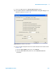


Table Of Contents
- Title Page
- Contents
- Getting Started
- Introduction and Measurement
- Phase Noise Basics
- Expanding Your Measurement Experience
- Starting the Measurement Software
- Using the Asset Manager
- Using the Server Hardware Connections to Specify the Source
- Setting GPIB Addresses
- Testing the 8663A Internal/External 10 MHz
- Testing the 8644B Internal/External 10 MHz
- Viewing Markers
- Omitting Spurs
- Displaying the Parameter Summary
- Exporting Measurement Results
- Absolute Measurement Fundamentals
- Absolute Measurement Examples
- Residual Measurement Fundamentals
- What is Residual Noise?
- Assumptions about Residual Phase Noise Measurements
- Calibrating the Measurement
- Measurement Difficulties
- Residual Measurement Examples
- FM Discriminator Fundamentals
- FM Discriminator Measurement Examples
- AM Noise Measurement Fundamentals
- AM Noise Measurement Examples
- Baseband Noise Measurement Examples
- Evaluating Your Measurement Results
- Advanced Software Features
- Reference Graphs and Tables
- Approximate System Noise Floor vs. R Port Signal Level
- Phase Noise Floor and Region of Validity
- Phase Noise Level of Various Agilent Sources
- Increase in Measured Noise as Ref Source Approaches DUT Noise
- Approximate Sensitivity of Delay Line Discriminator
- AM Calibration
- Voltage Controlled Source Tuning Requirements
- Tune Range of VCO for Center Voltage
- Peak Tuning Range Required by Noise Level
- Phase Lock Loop Bandwidth vs. Peak Tuning Range
- Noise Floor Limits Due to Peak Tuning Range
- Tuning Characteristics of Various VCO Source Options
- 8643A Frequency Limits
- 8644B Frequency Limits
- 8664A Frequency Limits
- 8665A Frequency Limits
- 8665B Frequency Limits
- System Specifications
- System Interconnections
- PC Components Installation
- Overview
- Step 1: Uninstall the current version of Agilent Technologies IO libraries
- Step 2: Uninstall all National Instruments products.
- Step 3: Install the National Instruments VXI software.
- Step 4: Install the National Instruments VISA runtime.
- Step 5: Install software for the NI Data Acquisition Software.
- Step 6: Hardware Installation
- Step 7. Finalize National Instruments Software Installation.
- Step 8: System Interconnections
- Step 9: Install Microsoft Visual C++ 2008 Redistributable Package use default settings
- Step 10: Install the Agilent I/O Libraries
- Step 11: Install the E5500 Phase Noise Measurement software.
- Step 12: Asset Configuration
- Step 13: License Key for the Phase Noise Test Set
- Overview
- PC Digitizer Performance Verification
- Preventive Maintenance
- Service, Support, and Safety Information
- Safety and Regulatory Information
- Safety summary
- Equipment Installation
- Environmental conditions
- Before applying power
- Ground the instrument or system
- Fuses and Circuit Breakers
- Maintenance
- Safety symbols and instrument markings
- Regulatory Compliance
- Declaration of Conformity
- Compliance with German noise requirements
- Compliance with Canadian EMC requirements
- Service and Support
- Return Procedure
- Safety and Regulatory Information
Residual Measurement Examples
8
Agilent E5505A User’s Guide 239
Making the measurement
Calibrate the measurement using measured ± DC peak voltage
Refer to Chapter 7, “Residual Measurement Fundamentals for more
information about residual phase noise measurements calibration types.
Procedure
1
Using Figure 173 and Figure 174 on page 240 as guides, connect the circuit
and tighten all connections.
2
Measure the power level that will be applied to the Signal Input port of the
test set phase detector. Table 37 shows the acceptable amplitude ranges for
the test set phase detectors.
Table 37 Acceptable amplitude ranges for the phase detectors
Phase Detector
50 kHz to 1.6 GHz
1.2 to 26.5 GHz
1
1 Phase Noise Test Set Options 001 and 201
Ref Input (L Port) Signal Input (R Port) Ref Input (L Port) Signal Input (R Port)
+
15 dBm
to
+
23 dBm
0 dBm
to
+
23 dBm
+
7 dBm
to
+
10 dBm
0 dBm
to
+
5 dBm
NOTE
Connecting an oscilloscope to the monitor port is recommended because the signal can
then be viewed to give visual confidence in the signal being measured. See Figure 173 and
Figure 174 on page 240.