
Operation Manual
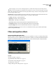
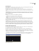
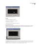
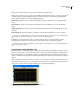
Table Of Contents
- Contents
- Chapter 1: Getting started
- Chapter 2: Digital audio fundamentals
- Chapter 3: Workflow and workspace
- Chapter 4: Setting up Adobe Audition
- Chapter 5: Importing, recording, and playing audio
- Chapter 6: Editing audio files
- Displaying audio in Edit View
- Selecting audio
- Copying, cutting, pasting, and deleting audio
- Visually fading and changing amplitude
- Working with markers
- Creating and deleting silence
- Inverting and reversing audio
- Generating audio
- Analyzing phase, frequency, and amplitude
- Converting sample types
- Recovery and undo
- Chapter 7: Applying effects
- Chapter 8: Effects reference
- Amplitude and compression effects
- Delay and echo effects
- Filter and equalizer effects
- Modulation effects
- Restoration effects
- Reverb effects
- Special effects
- Stereo imagery effects
- Changing stereo imagery
- Binaural Auto-Panner effect (Edit View only)
- Center Channel Extractor effect
- Channel Mixer effect
- Doppler Shifter effect (Edit View only)
- Graphic Panner effect
- Pan/Expand effect (Edit View only)
- Stereo Expander effect
- Stereo Field Rotate VST effect
- Stereo Field Rotate process effect (Edit View only)
- Time and pitch manipulation effects
- Multitrack effects
- Chapter 9: Mixing multitrack sessions
- Chapter 10: Composing with MIDI
- Chapter 11: Loops
- Chapter 12: Working with video
- Chapter 13: Creating surround sound
- Chapter 14: Saving and exporting
- Saving and exporting files
- Audio file formats
- About audio file formats
- 64-bit doubles (RAW) (.dbl)
- 8-bit signed (.sam)
- A/mu-Law Wave (.wav)
- ACM Waveform (.wav)
- Amiga IFF-8SVX (.iff, .svx)
- Apple AIFF (.aif, .snd)
- ASCII Text Data (.txt)
- Audition Loop (.cel)
- Creative Sound Blaster (.voc)
- Dialogic ADPCM (.vox)
- DiamondWare Digitized (.dwd)
- DVI/IMA ADPCM (.wav)
- Microsoft ADPCM (.wav)
- mp3PRO (.mp3)
- NeXT/Sun (.au, .snd)
- Ogg Vorbis (.ogg)
- SampleVision (.smp)
- Spectral Bitmap Image (.bmp)
- Windows Media Audio (.wma)
- Windows PCM (.wav, .bwf)
- PCM Raw Data (.pcm, .raw)
- Video file formats
- Adding file information
- Chapter 15: Automating tasks
- Chapter 16: Building audio CDs
- Chapter 17: Keyboard shortcuts
- Chapter 18: Digital audio glossary
- Index

ADOBE AUDITION 3.0
User Guide
130
See also
“About process effects” on page 104
“Apply individual effects in Edit View” on page 107
“Control effects settings with graphs” on page 104
“Use effect presets” on page 104
“Add preroll and postroll to effects previews” on page 107
FFT Filter options
Passive, Logarithmic modes Measures frequency changes (boosts or cuts) in percentages (Passive) or dB
(Logarithmic), where a setting of 100% or 0 dB represents no change.
View Initial Filter Graph, View Final Lets you set both an initial and a final filter setting if Lock To Constant Filter isn’t
selected. The rate at which the filter migrates from the initial to final settings depends on the Transition Curve
settings.
Log Scale Displays the x-axis (frequency) in a logarithmic scale rather than a linear scale. A logarithmic scale more
closely resembles the way the ear hears sound.
• To do finer editing in low frequencies, select Log Scale.
• For detailed, high-frequency work, or work with evenly spaced intervals in frequency, deselect Log Scale.
Max, Min Sets the maximum and minimum values for the horizontal ruler (y-axis).
FFT Size Specifies the size of the FFT to use (represented as a power of two), thereby affecting processing speed and
quality. For cleaner sounding filters, use higher values. Values between 1024 and 8192 work well.
Use a lower value (512 or so) for faster previews, and use a higher value after you achieve the settings you want for
better quality when processing audio.
Windowing Function Determines the amount of transition width and ripple cancellation that occurs during
filtering, with each one resulting in a different frequency response curve. These functions are listed in order from
smallest width and greatest ripples to widest and least ripples.
The filters with the least ripples are also those that most precisely follow the drawn graph and have the steepest
slopes, even though they are wider and pass more frequencies in a band-pass operation. The Hamming and
Blackman filters give excellent overall results.
Lock To Constant Filter Applies a constant filter to the waveform. Deselect this option to set initial and final filter
settings.
Morph Morphs the initial filter settings to the final filter settings. If this option is deselected, the settings simply
change in linear fashion over time. For example, if Morph is unselected, and you have a spike at 10 kHz for the initial
filterandaspikeat1kHzforthefinalfilter,thespikeat10kHzwillgraduallydecreaseovertime,andthespikeat1
kHz will gradually increase over time; frequencies between 1 kHz and 10 kHz won’t be affected. If Morph is selected,
however, the spike will gradually transition from 10 kHz down to 1 kHz, passing through the frequencies in between.
For a cool example of morphing, select Passive mode, and set an initial curve with the first half at 100% and the
second half at 0%. For the final curve, set the right tenth or so at 100% with the rest at 0%. This combination selects
high frequencies for the initial configuration, and low frequencies for the final configuration.
To get a nice blending from high to low, select Morph to include all the frequency combinations between the two
filters. Click Transition Curve to view the actual settings that will be used over the duration of the selection.